1. Introduction to Scientific Computing - - A Matrix Vector Approach Using Matlab Written by Charles F.Van Loan 陈 文 斌 Wbchen@fudan.edu.cn 复旦大学

2. Chapter3 Piecewise Polynomial Interpolation Piecewise Linear Interpolation Piecewise Cubic Hermite Interpolation Cubic Splines

3. 01234567 -0.8 -0.6 -0.4 -0.2 0 0.2 0.4 0.6 0.8 1 Piecewise Linear Interpolation

4. Piecewise Linear

5. function [a,b] = pwL(x,y) n = length(x); a = y(1:n-1); b = diff(y)./ diff(x); z=linspace(0,1,9); [a,b]=pwL(z,sin(2*pi*z)); for i=1:n-1 b(i)=(y(i+1)- y(i))/ (x(i+1)- x(i)); end b=(y(2:n)-y(1:n-1))./(x(2:n)-x(1:n- 1)) b=diff(y)./diff(x) Test code

6. Evalution Problem: if z==x(n) i =n-1; else i=sum(x<=z); end

7. Binary search mid = floor((Left+Right)/2); If z<x(mid) Right=mid; Else Left =mid; end

8. function i = Locate(x,z,g) % g (1<=g<=n-1) is an optional input parameter % search for i begins, the value i=g is tried. if nargin==3 if (x(g)<=z) & (z<=x(g+1)) i = g; return end;end n = length(x); if z = = x(n) i = n-1; else Left = 1; Right = n; while Right > Left+1 Binary_search end g: guss

9. function LVals = pwLEval(a,b,x,zVals) % Evaluates the piecewise linear polynomial defined by the column %(n-1)-vectors m = length(zVals); LVals = zeros(m,1); g = 1; for j=1:m i = Locate(x,zVals(j),g); LVals(j) = a(i) + b(i)*(zVals(j)-x(i)); g = i; end m-vector

11. A priori determination of breakpoints Static

12. Adaptive Piecewise Linear Interpolation Problem

13. Adaptive Piecewise Linear Interpolation acceptable or

17. Piecewise Cubic Hermit Interpolation

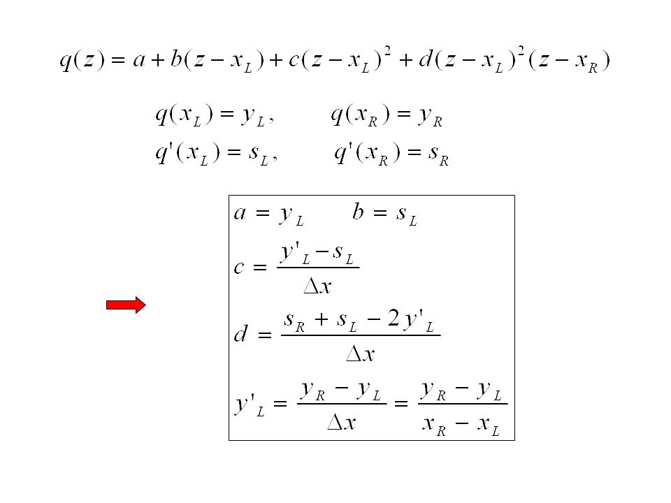
18. Hermit cubic interpolant

21. Piecewise cubic polynomial For i=1:n-1 [a(i),b(i), c(i), d(i)=Hcubic(x(i),y(i),s(i),x(i+1),y(i+1),s(i+1)) End

22. function [a,b,c,d] = pwC(x,y,s) % Piecewise cubic Hermite interpolation. n = length(x); a = y(1:n-1); b = s(1:n-1); Dx = diff(x); Dy = diff(y); yp = Dy./ Dx; c = (yp - s(1:n-1))./ Dx; d = (s(2:n) + s(1:n-1) - 2*yp)./ (Dx.* Dx); x,y,s: vector

23. Evaluation function Cvals = pwCEval(a,b,c,d,x,zVals) m = length(zVals); Cvals = zeros(m,1); g=1; for j=1:m i = Locate(x,zVals(j),g); Cvals(j) = d(i)*(zVals(j)-x(i+1)) + c(i); Cvals(j) = Cvals(j)*(zVals(j)-x(i)) + b(i); Cvals(j) = Cvals(j)*(zVals(j)-x(i)) + a(i); g = i; end Locate Cubic version of HornerN

25. Cubic spline interpolant Given with find a piecewise cubic interpolant with the property that S, S' and S'' are continuous. Why need spline?

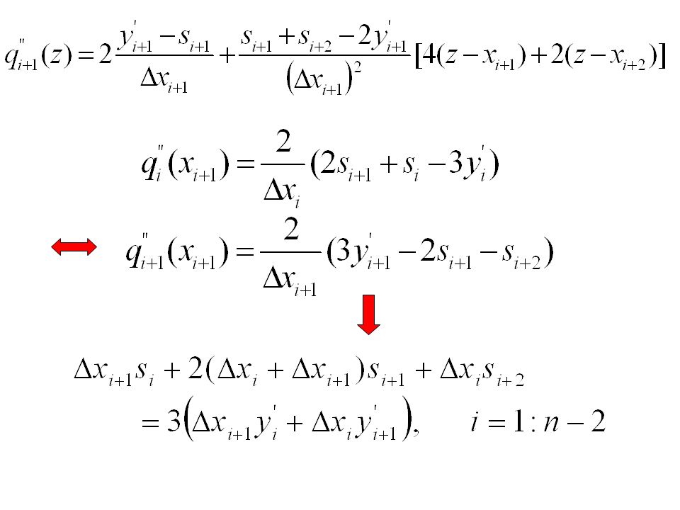
26. Continuity at the interior knots

29. tridiagonal

30. choice

31. n=length(x); Dx=diff(x); yp=diff(y)./Dx; T=zeros(n-2,n-2); r=zeros(n-2,1); for i=2:n-3 T(i,i)=2(Dx(i)+Dx(i+1)); T(i,i-1)=Dx(i+1); T(i,i+1)=Dx(i); r(i)=3(Dx(i+1)*yp(i)+Dx(i)*yp(i+1)); end Help diag

32. The complete spline

33. T(1,1)=2*(Dx(1)+Dx(2)); T(1,2)=Dx(1); r(1)=3*(Dx(2)*yp(1)+Dx(1)*yp(2))-Dx(2)*muL; T(n-2,n-2)=2*(Dx(n-2)+Dx(n-1)); T(n-2,n-3)=Dx(n-1); r(n-2)=3*(Dx(n-1)*yp(n-2)+Dx(n-2)*yp(n-1))-Dx(n-2)*muR; s=[muL;T\r(1:n-2);muR];

34. The Natural Spline

35. T(1,1) = 2*Dx(1) + 1.5*Dx(2); T(1,2) = Dx(1); r(1) = 1.5*Dx(2)*yp(1) + 3*Dx(1)*yp(2) + Dx(1)*Dx(2)*muL/4; T(n-2,n-2) = 1.5*Dx(n-2)+2*Dx(n-1); T(n-2,n-3) = Dx(n-1); r(n-2) = 3*Dx(n-1)*yp(n-2) + 1.5*Dx(n-2)*yp(n-1)- … Dx(n-1)*Dx(n-2)*muR/4; stilde = T\r; s1 = (3*yp(1) - stilde(1) - muL*Dx(1)/2)/2; sn = (3*yp(n-1) - stilde(n-2) + muR*Dx(n-1)/2)/2; s = [s1;stilde;sn];

36. The Not-a-Knot Spline

37. q = Dx(1)*Dx(1)/Dx(2); T(1,1) = 2*Dx(1) +Dx(2) + q; T(1,2) = Dx(1) + q; r(1) = Dx(2)*yp(1) + Dx(1)*yp(2)+2*yp(2)*(q+Dx(1)); q = Dx(n-1)*Dx(n-1)/Dx(n-2); T(n-2,n-2) = 2*Dx(n-1) + Dx(n-2)+q; T(n-2,n-3) = Dx(n-1)+q; r(n-2) = Dx(n-1)*yp(n-2) + Dx(n-2)*yp(n-1) … +2*yp(n-2)*(Dx(n-1)+q); stilde = T\r; s1 = -stilde(1)+2*yp(1); s1 = s1 + ((Dx(1)/Dx(2))^2)*(stilde(1)+stilde(2)-2*yp(2)); sn = -stilde(n-2) +2*yp(n-1); sn = sn+((Dx(n-1)/Dx(n-2))^2)*(stilde(n-3) … +stilde(n-2)-2*yp(n-2)); s = [s1;stilde;sn];

38. function [a,b,c,d] = CubicSpline(x,y,derivative,muL,muR) % Cubic spline interpolation with prescribed end conditions. % Usage: % [a,b,c,d] = CubicSpline(x,y,1,muL,muR) % S'(x(1)) = muL, S'(x(n)) = muR % [a,b,c,d] = CubicSpline(x,y,2,muL,muR) % S''(x(1)) = muL, S''(x(n)) = muR % [a,b,c,d] = CubicSpline(x,y) % S'''(z) continuous at x(2) and x(n-1)

39. 10 -10 10 -8 10 -6 10 -4 Knot Spacing = 0.005 Not-a-knot spline error

40. 012345678910 -0.5 0 0.5 1 1.5 Bad end conditions

41. -5-4-3-2012345 -1.5 -0.5 0 0.5 1 1.5 n = 9 Spline Interpolant of atan(x) Matlab Spline Tools z=linspace(-5,5); x=linspace(-5,5,9); y=atan(x); Svals=spline(x,y,z); plot(z,Svals) Not-a-knot spline

42. pp-representation x=linspace(-5,5,9); y=atan(x); S=spline(x,y); z=linspace(-5,5); Svals=ppval(S,z) plot(z,Svals) pp-representation [x, rho,L,k]=unmkpp(S) The coefficients of the local polynomials are assembled in an L-by-k matrix rho

43. drho = [3*rho(:,1) 2*rho(:,2) rho(:,3)]; dS = mkpp(x,drho); V = PPVAL(PP,XX) returns the value at the points XX of the piecewise polynomial contained in PP, as constructed by SPLINE or the spline utility z = linspace(-5,5); Svals = ppval(S,z); dSvals = ppval(dS,z);

44. -5-4-3-2012345 0 0.1 0.2 0.3 0.4 0.5 0.6 0.7 0.8 0.9 1 Derivative of n = 9 Spline Interpolant of atan(x)

45. n = 9;x = linspace(-5,5,n);y = atan(x);S = spline(x,y); [x,rho,L,k] = unmkpp(S); drho = [3*rho(:,1) 2*rho(:,2) rho(:,3)]; dS = mkpp(x,drho); z = linspace(-5,5); Svals = ppval(S,z); dSvals = ppval(dS,z); atanvals = atan(z); Figure;plot(z,atanvals,z,Svals,x,y,'*'); title(sprintf('n = %2.0f Spline Interpolant of atan(x)',n)) datanvals = ones(size(z))./(1 + z.*z); figure plot(z,datanvals,z,dSvals) title(sprintf('Derivative of n = %2.0f Spline Interpolant of atan(x)',n))