1. Church’s Problem and a Tour through Automata Theory Wolfgang Thomas Pillars of Computer Science. Springer Berlin Heidelberg, 2008

2. Church’s problem Stated by Alonzo Church in 1957: Given a requirement which a circuit is to satisfy, we may suppose the requirement expressed in some suitable logistic system which is an extension of restricted recursive arithmetic. The synthesis problem is then to find recursion equivalences representing a circuit that satisfies the given requirement (or alternatively, to determine that there is no such circuit) The requirement taken as transformation from one infinite bit string to anothe r – Transforming every α to β such that holds – Transformations expected to be nonaticipatory and computable with finite memory – Finite state automata replaces logical circuits

3. Mealy automaton (reminder) A tuple M=(S,Σ, Γ, s 0, δ, τ) – S is the finite set of states – s 0 is the initial state – Σ is the finite input alphabet – Γ is the finite output alphabet – δ: S × Σ → S is the transition function – τ : S × Σ → Γ is the output function – f M : Σ ω → Γ ω defined as the transformation computed by M

4. “Some suitable logistic system”

5. Logistic systems Propositional  First-order  Second-order logics Propositional logic: – Propositional variables with boolean operators First-order logic: – Atomic formulae Variables + Functions +constants  terms Relations over terms – Boolean operators – Quantifiers over variables – Models/structures Monadic second-order logic: – First-order logic with: relations and functions as variables (special case - sets) Quantification over set variables

6. S1S logic Stands for “second-order theory of one successor” Monadic second-order logic over ( ℕ,+1,<,0) Includes numbers and sets as variables Allows for formulae such as: –.

7. Church’s problem in S1S A bit string α can be represented by the relation X such that α[i]=1 iff X(i) Consequently, in S1S bit strings can be quantified variables By extention, tuples of bit strings can be formulated as variables Church’s problem restated: Solved in 1967 by Buchi and Landweber We’ll follow the proof for m1=m2=1

8. Church problem - example Under the hood:

9. Following the proof S1S specification  Deterministic Muller Deterministic Muller  Muller game graph Muller game graph  Parity game graph Parity game graph  Winning strategy Winning strategy  Mealy automaton

10. Deterministic Muller automaton (reminder) A tuple M=(S,Σ, s 0, δ, F) – S is the finite set of states – s 0 is the initial state – Σ is the finite input alphabet – δ: Q × Σ → Q is the transition function – is the acceptance condition A run ρ=(r 0,…) on a=(a 0,…) is a sequence s.t. r 0 = s 0, r i = δ(r i-1,a i ) The infinite states of a run - M accepts a iff inf(ρ) is in F

11. Nondeterministic Muller automaton (reminder) A tuple M=(S,Σ, S 0, Δ, F) – S 0 is a set of initial states – Δ : Q × Σ → P(Q) is the transition function – A run ρ=(r 0,…) on a=(a 0,…) is a sequence s.t. r 0 = s 0, Δ (r i-1,a i ) ∈ r i – M accepts a if an accepting run on a exists

12. From S1S to Muller Let ф(X,Y) be a formula in S1S with free variables X,Y representing the strings α,β We will construct a deterministic Muller automaton running on the input ((α 0,β 0 ), (α 1,β 1 ),…) First, let’s express the relation ‘>‘ with the other S1S constructs a < b equivalent to. Not in paper

13. From S1S to Muller We can also express free number variables in term of sets: –. – Allows for intentional omitting in the proof And define 0 General case - ф(x 1,…,x k, Y 1,…, Y n ) w.l.o.g., all atomic formulae are of form – Z(S k a), for some k The rest, by structural induction, on board

14. Following the proof (recap) S1S specification  Deterministic Muller ✓ Deterministic Muller  Muller game graph Muller game graph  Parity game graph Parity game graph  Winning strategy Winning strategy  Mealy automaton

15. From Muller automata to Muller game Given a Muller automata expressing ф, with input ((α 0,β 0 ), (α 1,β 1 ),…), construct an equivalent automata on input (α 0,β 0, α 1,β 1,…) Admits a partition of S to S α and S β

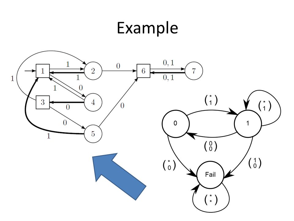
16. Example

18. From Muller automata to Muller game The equivalent automata defines a game The arena is the state graph, denoted G=(Q,Q A,E) Note that each node has nonzero out degree – A subgraph with Q 0 is a game iff there’s an edge to Q 0 from every q in Q 0 The winning condition: – Define F by identifying each original node with its Q A equivalent – Player B wins play ρ iff F ∈ Inf(ρ)

19. Following the proof (recap) S1S specification  Deterministic Muller ✓ Deterministic Muller  Muller game graph ✓ Muller game graph  Parity game graph Parity game graph  Winning strategy Winning strategy  Mealy automaton

20. Solving graph games A strategy for player B from q is a function f:Q + → Q s.t. for any prefix q 0,…,q k with q 0 =q and q k in Q B,E ∈ f(q 0,…,q k ) A play ρ= q 0,… is played according to f iff A winning strategy is such that any game played by it results in a win for player B W A and W B Are the states from which players A,B have a winning strategy

21. Solving graph games A game is called determined if W A ∪ W B =G. Solving a game involves two tasks: – Deciding, for each state q, if it’s a winning state for one of the players – If so, constructing a winning strategy from q A winning strategy f is finite-state if it can be computed by a mealy automaton

22. Warming up – Reachability games Let’s explorer a simpler type of games before On a reachability game, player B wins if the play passes through a state in F Define F’s ‘attractors’:

23. Warming up – Reachability games Define It holds that Attr B (F)=W B Furthermore, the recursive definition of Attr B admits a memoryless winning strategy from every q in W B G ∖ W B =W A, and therefore, reachability games are decideable And we’ve now shown they’re solvable

24. Appearance records Memoryless strategies are not enough for Muller games Consider this example, with F={{1,2,3}} Define Occ(ρ) as the set of states that are encountered in ρ The weak Muller game requires Occ(ρ) in F Still not solvable with memoryless strategies

25. Weak Muller games We can solve weak Muller games with a finite state strategy Define S with states P(Q), and Q as input alphabet The transition function is δ:P(Q) × Q → P(Q) defined by δ(R, p) = R ∪ {p} This memory structure is called appearance record

26. Strong Muller games For strong Muller games a stronger memory structure is required (by McNaughton) Recall Latest Appearance Records, or LAR: – A LAR is a pair ((q 1,..., q r ), h), with q j being distinct states and 0≥h≥r – The initial state is ((),0) – On input q, supposing q appears in the LAR with index j, the new LAR will be ((q 1,..., q r q,j)

27. From Muller games to Parity games Consider the appearance record (AR) of a weak Muller game If R=(R 1,…,R k ) is a prefix of T, then AR(R) ⊇ AR(T) For R n the n’th prefix of a game ρ, Lim n->∞ AR(R n ) = Occ(ρ) AR reaches Occ(ρ) in finite steps, and halts there

28. From Muller games to Parity games Accociate a number c(R) with R in P(Q), that reports both its size, and membership in F A play ρ admits the sequence c(AR(p i )) Note that the inclusion relation agrees with the order on c(R) Then, Occ(ρ) is in F iff the maximal number in the sequence is even

29. From Muller games to Parity games A weak parity game is a game with a numbering of Q, with the following winning condition: – Max(c(p i )|p i ⊇ ρ) is even Now we can transform a weak Muller game to a weak parity game: –. – c as defined previously This transformation is called “game simulation”, as it transforms winning plays to winning plays

30. From Muller games to Parity games A regular parity game has the following winning condition: – The maximal number c(p) that occurs infinitely often is even Now we can transform a Muller game to a parity game: – Define as the set of ordered subsets of Q –.

31. From Muller games to Parity games For a LAR ((q 1,..., q r ), h), denote h the ‘hit’ and {q 1,...,q h } as the ‘hit set’ Denote the maximal hit encountered infinitely often in a run ρ as h ρ Recall this property of LARs previously proven: – ∃ i s.t. hit sets of size h ρ for all p j>I are identical – Hit sets of size h ρ occur infinitely often – Thus, the repeating maximal hit set is Inf(ρ) Therefore, the transformation is a game simulation

32. Following the proof (recap) S1S specification  Deterministic Muller ✓ Deterministic Muller  Muller game graph ✓ Muller game graph  Parity game graph ✓ Parity game graph  Winning strategy Winning strategy  Mealy automaton

33. Solving weak parity games It will be now shown that weak parity games are determined, and solvable with finite memory Let G=(Q,Q A,E) be a weak parity game with coloring c:Q→ {0,..., k} (w.l.o.g k even) Define C i ={q ∈ Q | c(q) = i} Denote A k =Attr B (C k ). It holds that A k ⊇ W B Argue that Q ∖ A k is a game graph (out degree)

34. Solving weak parity games Denote As the set of states in the subgraph From which player B can force the play to Continue defining recursively:

35. Solving weak parity games It holds that For each subgraph G i, winning strategies for players A,B are determined by the construction of the attractors Together they constitute a global finite memory winning strategy from every winning state

36. Solving regular parity games It is left to show that regular parity games are determined, and admit finite memory winning strategies (proof due to McNaughton) Proof by induction on the size of G For a singleton G, trivial For the induction step, assume w.l.o.g k is even (otherwise raise c by one, and switch roles)

37. Solving regular parity games Let q be a highest-number state and define A 0 =Attr B ({q}). The remaining graph is again a subgame From the induction hypothesis, one can partition it to winning regions U A,U B with finite memory winning strategies There are then two possible cases: – From q, player B can ensure to be in U B ∪ A 0 in the next step, – From q, player A can ensure to be in U A in the next step.

38. Solving regular parity games For case 1, we will show W B = U B ∪ A 0,W A = U A A play from U B ∪ A 0 either: – remains in U b from some point onwards, which admits a finite memory winning strategy to player B by induction hypothesis – Visits A 0 infinitely often, from which player be can ensure infinite visits to q (highest even number) Thus, player B has a finite memory winning strategy from all states in U B ∪ A 0, composed of the strategies for U B, A 0, and (possibly) the edge from q to A 0

39. Solving regular parity games For case 2, note that q ∈ Attr A (U A ) Thus, A1 = Attr A (U A ) is of cardinality 1≤ We can then use the induction hypothesis on Q\A1, getting a partitioning to V A,V B By repeating the same arguments, one gets W B = V B,W A = V A ∪ A 1 Similarly, a memoryless strategy can be constructed for player A

40. Church’s problem We have transformed the setting of church’s problem to first a Muller game, and subsequently an equivalent parity game The recursive build of the Attractors provides an algorithm for computing winning regions and finite memory winning strategies A mealy automaton playing the simulated game can output the desired bit string – Winning the parity game  winning the Muller game – Winning the Muller game  Moves of B player constitute a legal β string