1. Search for bursts with the Frequency Domain Adaptive Filter (FDAF ) Sabrina D’Antonio Roma II Tor Vergata Sergio Frasca, Pia Astone Roma 1 Outlines: FDAF description FDAF description Project1a data application Project1a data application Filters performances comparison Filters performances comparison WSR7 seg. 27 data application WSR7 seg. 27 data application

2. Overview on the filter and cluster generation procedure Three STEPS: 1. Filtering procedure: An Adaptive Wiener Filter (AWF), in frequency domain, followed by a series (N) of band-pass filters with a Gaussian shape (phase zero) ->(N+1) filtered output 2. Event extraction An Adaptive threshold algorithm for the selection of the events applied at each filtered channel CH (N+1). 3. Cluster generation Events coming from different CH in coincidence in a given time window W are put together: this is one CLUSTER

3. RAW DATA Wiener Filter WF Power Spectrum SP estimation Filters bank (N) With Gaussian shape FFT 1 2..... 4....... …... ….. N+1 filtered output channels In the time domain Filtering procedure IFFT Hp Frequency domain back in time-domain Hp

4. Power spectra estimation PS is the estimated Power Spectrum of the noise, evaluated with a first order Auto-Regressive (AR) sum of the periodograms, P i : from PS i ’ = W ∙ PS’ i-1 + P i and n i = 1 + W ∙ n i-1 PS=PS’/n in our case: W=exp(-T/tau)= 0.9991 T= 3.2768 s (time duration of one data chunk used to obtain the Periodogram) tau=3600 s (Memory time: Simulated data-> stationary noise)

5. Event extraction: adaptive threshold technique for the events selection ( event search procedure applied at each filtered channel y(i)) Let y(i) the filtered data samples in time domain, we estimate m i = y i + W∙m i-1 q i = y² i + W∙q i-1 n i = 1 + W∙n i-1 with W = exp(-dt/tau) = 0.9999900 (corresponding to dt= 1/20000 s & tau = 5 s) and M i = m i /n I Q i = q i /n i S i = sqrt(Q i -(M i ) 2 ) From these we define the Critical Ratio (CR i ) of y(i) CR i =|(y i -M i )/S i |

6. Event extraction We define a “dead time’’, t d, as the minimum time between two events, and we put the threshold, ϑ, on the CR. A two-state ( 0 and 1 ) mechanism “event machine’’ has been used: 1. The “machine’’ starts with state 0 2. When CR > ϑ, it changes to state 1 and an event begins 3. The state changes to 0 after CR remains below ϑ for a time > t d (the event finishes) T0 = starting time CRmax = Max value of CR A = amplitude The ‘event’ is characterized Tmax = time of max CR by: L = length (in seconds) (duration of state 1) CH = frequency channel ϑ =3.9 td=0.2 s

7. Event cluster EVENT LIST of all frequency Channel (N+1) Ch1 Time CR … … … Ch4 Time CR … … … Ch7 Time CR … … … ……………… ………………… … … …………………………. Ch1 Time CR All Events coming from different frequency channel Ch in coincidences into a given time window W are put together: this is one CLUSTER. The time corresponding to the higher CR is the CLUSTER time. CLUSTER list Time CR1 CR2 CR3 …. CRN+1 Time CR1 … … … CRN+1 …………………. Time CR1 … … … CRN+1 CR i =0 if the frequency channel Ch i not in time coincidence with other.

8. Event cluster example (Preliminary Procedure!) Frequency channels: Mean values of the Gaussian filters CR value WF channel 0-2000 Hz Event list: Freq. Channel Time cr Ampl length.. 1 (40 Hz) tim1 6.13 … ….... ….... 2 (90Hz) tim2 6.75 … ….... ….. 3 (200Hz) tim3 6.0 … ….... ….... 10(0-2000Hz) tim10 4.8 6 … … Time distances tim10-tim1 < W=10ms They are put together-> one CLUSTER Cluster list Time CR1 CR2 CR3 CR4........ CR10 Time2 6.13 6.75 6.0 0 0 0 0 0 4.8 cluster ordering number CR 40 90 200 600 1000 1400 0-2000 Hz tim2 is the time corresponding to the maximum CR ->time2=CLUSTER time

9. Project1a preliminary results gr-qc/0701026 A comparison of methods for gravitational wave burst searches from LIGO and Virgo

10. 3 hours of Virgo simulated noise

11. Injected signals INPUT: 3 hours of Virgo (vs=20 kHz) simulated noise Signals injected with SNR=7, 10 Gaussian signals with σ = 1ms 2 kinds of supernovae signals (from Dimmelmeier-Font-Muller simulations) @ 8.5 kpc: A1B2G1,A2B4G1) Sine-Gaussian signals with Q = 5 and ν = 235 Hz or ν = 820 Hz Sine-Gaussian signals with Q = 15 and ν = 820 Hz Wiener filter (WF) +Band-Pass filters with Gaussian shape: The frequency range 0-2000 Hz is linearly divided into 9 bands (step = 200 Hz, Sigma=100 Hz). --> 10 different filters

12. Waveform families of burst sources used in this study: time domain

13. Waveform families of burst sources used in this study: frequency domain

14. SGQ15f820: clusters in time coincidences with the injected signals (163) at SNR=7 (frequency domain characteristic) Due to the noise! Not in the expected channel and they don’t change with the SNR of injected signals SNR=7: CR SNR=7: number of event detected from each channel cluster ordering number Event number 90 200 600 1000 1400 0-2000 Hz

15. SGQ15f820: clusters in time coincidences with the injected signals (163) at SNR=10 (frequency domain characteristic) Due to the noise! Not in the expected channel and they don’t change with the SNR of injected signals N SNR=10: CR cluster ordering number 90 200 600 1000 1400 0-2000 Hz SNR=10: number of event detected from each channel Event number 90 200 600 1000 1400 0-2000 Hz

16. SGQ5f820: clusterin time coincidences with the injected signals (178) at SNR=7 (frequency domain characteristic) SNR=7: CR cluster ordering number 90 200 600 1000 1400 0-2000 Hz SNR=7: number of event detected from each channel Event number 90 200 600 1000 1400 0-2000 Hz

17. SGQ5f820: cluster in time coincidences with the injected signals (178) at SNR=10 (frequency domain characteristic) SNR=10: CR cluster ordering number 90 200 600 1000 1400 0-2000 Hz SNR=10: number of event detected from each channel Event number 90 200 600 1000 1400 0-2000 Hz

18. SGQ5f235: clusters in time coincidences with the injected signals (190) at SNR=7 (frequency domain characteristic) SNR=7: CR cluster ordering number 90 200 600 1000 1400 0-2000 Hz SNR=7: number of event detected from each channel Event number 90 200 600 1000 1400 0-2000 Hz

19. SGQ5f235: clusters in time coincidences with the injected signals (190) at SNR=10 (frequency domain characteristic) SNR=10: CR cluster ordering number 90 200 600 1000 1400 0-2000 Hz SNR=10: number of event detected from each channel Event number 90 200 600 1000 1400 0-2000 Hz

20. A1B2G1: clusters in time coincidences with the injected signals (165) at SNR=7 (frequency domain characteristic) SNR=7: CR cluster ordering number 90 200 600 1000 1400 0-2000 Hz SNR=7: number of event detected from each channel Event number 90 200 600 1000 1400 0-2000 Hz

21. A1B2G1: clusters in time coincidences with the injected signals (165) at SNR=10 (frequency domain characteristic) SNR=10: CR cluster ordering number 90 200 600 1000 1400 0-2000 Hz SNR=10: number of event detected from each channel Event number 90 200 600 1000 1400 0-2000 Hz

22. A2B4G1: clusters in time coincidences with the injected signals (170) at SNR=7 (frequency domain characteristic) SNR=7: CR cluster ordering number 90 200 600 1000 1400 0-2000 Hz SNR=7: number of event detected from each channel Event number 90 200 600 1000 1400 0-2000 Hz

23. A2B4G1: clusters in time coincidences with the injected signals (170) at SNR=10 (frequency domain characteristic) SNR=10: CR cluster ordering number 90 200 600 1000 1400 0-2000 Hz SNR=10: number of event detected from each channel Event number 90 200 600 1000 1400 0-2000 Hz

24. To see better the lower frequency region (A2B4G1 & GAUSS1ms) I’ve added another channel at 40 Hz

25. A2B4G1: clusters in time coincidences with the injected signals (170) at SNR=7 (frequency domain characteristic) SNR=7: CR cluster ordering number 40 90 200 600 1000 0-2000 Hz SNR=7: number of event detected from each channel Event number 40 90 200 600 1000 0-2000 Hz

26. A2B4G1: clusters in time coincidences with the injected signals (170) at SNR=10 (frequency domain characteristic) SNR=10: CR cluster ordering number SNR=10: number of event detected from each channel Event number 40 90 200 600 1000 0-2000 Hz

27. GAU1ms: clusters in time coincidences with the injected signals (178) at SNR=7 (frequency domain characteristic) SNR=7: CR cluster ordering number 40 90 200 600 1000 0-2000 Hz SNR=7: number of event detected from each channel Event number 40 90 200 600 1000 0-2000 Hz

28. GAU1ms: clusters in time coincidences with the injected signals (178) at SNR=10 (frequency domain characteristic) SNR=10: CR cluster ordering number 40 90 200 600 1000 0-2000 Hz SNR=10: number of event detected from each channel Event number 40 90 200 600 1000 0-2000 Hz

29. Trigger due to the noise (no signal injection!) NOISE: CR cluster ordering number NOISE: number of event in each channel Event number 90 200 600 1000 1400 0-2000 Hz

30. SignalSNR Std(CR)bias [ms] Std(DT) [ms] Eff % SGQ15f820108.98 @(4.2) 1.0 @(0.46) -0.031 *35.6% 0.55100 76.42 (4.2) 0.94 (0.3) -0.06 *20.86% 0.8100 A1B2G1108.28 (4.2) 1.0 (0.4) -0.008 *43% 0.05100 75.92 (4.2) 0.9 (0.3) -0.0024 *32.5% 0.198.2 SGQ5f820108.3 (4.2) 1.0 (0.4) -0.008 *55% 0.26100 75.99 (4.2) 0.9 (0.3) 0.0 *34.3% 0.3997.8 * : percentage of CLUSTERS detected at the exact sample (DT=0.0) @: obtained over all CLUSTERS (due to the noise+ due to the signals)

31. SignalSNR Std(CR)bias [ms] Std(DT) [ms] Eff % SGQ5f235108.24 (4.2) 1.0 (0.4) 0.1 *24.21% 0.8100 99.4 75.99 (4.2) 1.0 (0.3) 0.006 *15.22% 1.296.84 A2B4G1106.4 7.47 (4.2) 0.9 (0.4) 0.8 1.0 0.96 0.28 100 74.86 5.36 (4.2) 0.64 0.8 (0.3) 0.85 1.0 1.5 0.9 78.8 97.05 GAUSS1ms108.9 (4.2) 1.0 (0.5) -0.007 *18% 0.11100 76.3 (4.2) 0.9 (0.3) -0.015 *11.3% 0.1799.4 *: percentage of CLUSTERS detected at the exact sample (DT=0.0) The red values are obtained adding the lower frequency channel at 40 Hz

32. Filters performances comparison

33. Efficiency vs False Alarm Rate SNR=7 (Comparison with Power filter (Red)) sgQ15f820 A1B2G1 GAU1ms A2B4G1

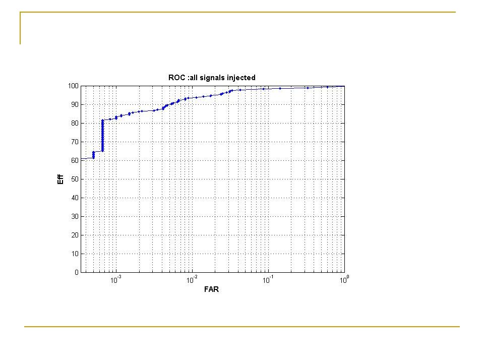
34. sgQ5f235 sgQ5f820 Signals injected with SNR=10 give efficiency=1 with FAR=10 -4 Efficiency vs False Alarm Rate SNR=7

35. Time error comparison std[ms] Std[ms] QTPFKWPCEGCMFALFAFDF A1B2G1 0.20.050.50.040.030.050.30.05 A2B4G1 1.40.72.60.20.40.52.20.28 GAUSS1 0.81.21.40.10.20.81.50.11 SG235Q5 0.91.40.91.30.51.31.10.8 SG820Q5 0.2 0.3-0.20.3 0.26 SG820Q15 0.70.61.1-0.51.31.10.55

36. Time error comparison bias [ms] bias[ms] QTPFKWPCEGCMFALFAFDF A1B2G1 -0.10.20.3-0.05-0.060.030.1-0.008 A2B4G1 -1.71.94.9-1.3-1.42.10.7 1.0 GAUSS1 -0.051.73.4-0.010.012.31.7-0.007 SG235Q5 -0.070.61.30.02 0.7 0.1 SG820Q5 -0.010.2 -0.010.1 -0.008 SG820Q15 -0.040.20.3-0.030.30.2-0.031

37. WSR7 Preliminary Results seg.27 GPS time start=852852866 GPS time stop =852858889 Hardware Injections: (SNR=7.5,15,25) Injected signals N SGf1000Q5/Q15 34/34 SGf1300Q5/Q15 34/34 SGf1600Q5/Q15 34/33 = 271 inj. GAUSSIAN 34/34 A2B4G1 34/34

38. Pre HP filter with freq. cutoff at 80 Hz Power Spectra Estimation: tau=1800 s T=3.2768 s CR: ϑ =4.0 Wiener filter (WF) +Band-Pass filters with Gaussian shape: The frequency range 0-2000 Hz is linearly divided into 10 bands (step = 150 Hz, Sigma=100 Hz). --> 11 different filters

39. GAUSSIAN/A2B4G1: all signals detected 150 550 800 1150 1450 0-2000 Hz

40. SGf1000Q15/Q5: all signals detected 150 550 800 1150 1450 0-2000 Hz

41. SGf1300Q15/Q5: all signals detected 150 550 800 1150 1450 0-2000 Hz

42. SGf1600Q15/Q5: all events detected 150 550 800 1150 1450 0-2000 Hz

43. Signal Std(CR/SNR)Bias [ms] Std(DT) [ms] Eff % SGf1000Q150.990.11-0.670.38100 SGf1000Q50.970.11-0.540.22100 SGf1300Q151.150.11-0.890.41100 SGf1300Q50.90.10-0.70.39100 SGf1600Q151.220.10-0.50.38100 SGf1600Q50.90.12-0.540.38100 A2B4G10.70.1-2.30.8100 GAUSSIAN0.920.088-0.450.1100

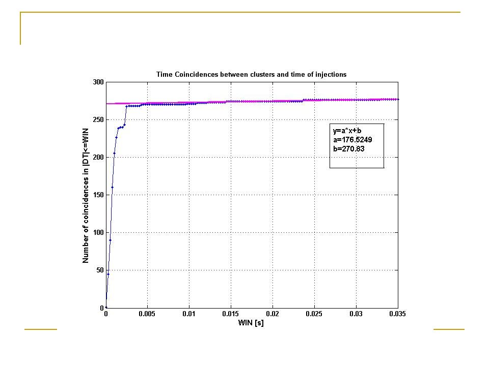
44. CR: clusters in time coincidence with the injected signals all clusters-271 clusters in time coincidence with the injected signals =15.22 Std(CR)=7.27 =4.44 Std(CR)=0.61

45. 4 BIG events not due to the injected signals (first injection time=852852651.45370)

48. Without 4 big events

50. Signal Dt=1/20000 [s] Std(CR/SNR)Bias [ms] Std(DT) [ms] Eff % SGf1000Q150.9960.116-0.560.31100 SGf1000Q50.970.11-0.570.15100 SGf1300Q151.150.11-0.970.32100 SGf1300Q50.90.10-0.620.15100 SGf1600Q151.220.10-0.550.15100 SGf1600Q50.90.12-0.540.17100 A2B4G10.70.1-2.30.8100 GAUSSIAN0.920.09-0.450.0065100