1. Statistical tests for Quantitative variables (z-test, t-test & Correlation) BY Dr.Shaikh Shaffi Ahamed Ph.D., Associate Professor Dept. of Family & Community Medicine College of Medicine, King Saud University

2. Objectives: (1) Able to understand the factors to apply for the choice of statistical tests in analyzing the data. (2) Able to apply appropriately Z-test, student’s t-test & Correlation (3) Able to interpret the findings of the analysis using these three tests.

3. Choosing the appropriate Statistical test Based on the three aspects of the data Type of variables Number of groups being compared & Sample size

4. Statistical Tests Z-test: Study variable: Qualitative (Categorical) Outcome variable: Quantitative Comparison: (i)sample mean with population mean (ii)two sample means Sample size: larger in each group(>30) & standard deviation is known

5. Steps for Hypothesis Testing Draw Research Conclusion Formulate H 0 and H 1 Select Appropriate Test Choose Level of Significance (3) Determine Prob Assoc with Test Stat (1)Determine Critical Value of Test Stat TS CR (2) Determine if TS CR falls into (Non) Rejection Region (4) Compare with Level of Significance,  Reject/Do not Reject H 0 Calculate Test Statistic TS CAL

6. Example( Comparing Sample mean with Population mean): The education department at a university has been accused of “grade inflation” in medical students with higher GPAs than students in general. GPAs of all medical students should be compared with the GPAs of all other (non-medical) students. –There are 1000s of medical students, far too many to interview. –How can this be investigated without interviewing all medical students ?

7. What we know: The average GPA for all students is 2.70. This value is a parameter. To the right is the statistical information for a random sample of medical students:  = 2.70 =3.00 s =0.70 n =117

8. Questions to ask: Is there a difference between the parameter (2.70) and the statistic (3.00)? Could the observed difference have been caused by random chance? Is the difference real (significant)?

9. 1.The sample mean (3.00) is the same as the pop. mean (2.70). –The difference is trivial and caused by random chance. 2.The difference is real (significant). –Medical students are different from all other students.

10. Step 1: Make Assumptions and Meet Test Requirements Random sampling  Hypothesis testing assumes samples were selected using random sampling.  In this case, the sample of 117 cases was randomly selected from all medical students. Level of Measurement is Interval-Ratio  GPA is I-R so the mean is an appropriate statistic. Sampling Distribution is normal in shape  This is a “large” sample (n≥100).

11. Step 2 State the Null Hypothesis H 0 : μ = 2.7 (in other words, H 0 : = μ)  You can also state H o : No difference between the sample mean and the population parameter  (In other words, the sample mean of 3.0 really the same as the population mean of 2.7 – the difference is not real but is due to chance.)  The sample of 117 comes from a population that has a GPA of 2.7.  The difference between 2.7 and 3.0 is trivial and caused by random chance.

12. Step 2 (cont.) State the Alternat Hypothesis H 1 : μ≠2.7 (or, H 0 : ≠ μ)  Or H 1 : There is a difference between the sample mean and the population parameter  The sample of 117 comes a population that does not have a GPA of 2.7. In reality, it comes from a different population.  The difference between 2.7 and 3.0 reflects an actual difference between medical students and other students.  Note that we are testing whether the population the sample comes from is from a different population or is the same as the general student population.

13. Step 3 Select Sampling Distribution and Establish the Critical Region Sampling Distribution= Z  Alpha (α) =.05  α is the indicator of “rare” events.  Any difference with a probability less than α is rare and will cause us to reject the H 0.

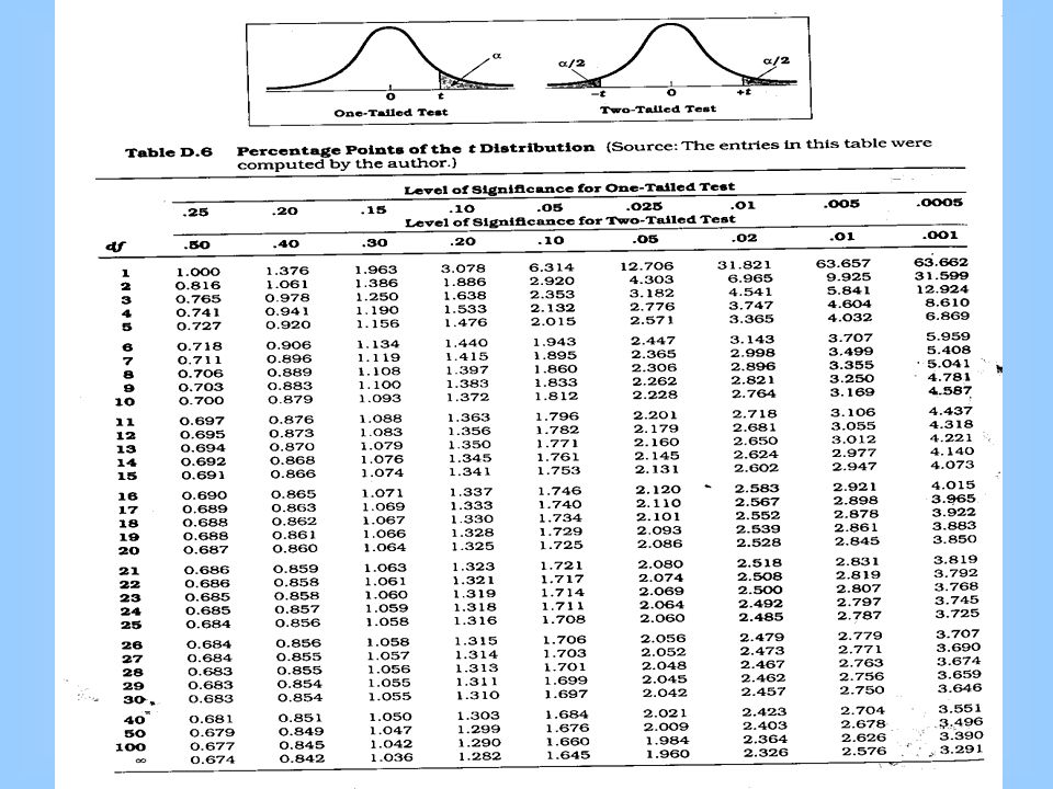
14. Step 3 (cont.) Select Sampling Distribution and Establish the Critical Region Critical Region begins at Z= ± 1.96  This is the critical Z score associated with α =.05, two-tailed test.  If the obtained Z score falls in the Critical Region, or “the region of rejection,” then we would reject the H 0.

15. Step 4: Use Formula to Compute the Test Statistic (Z for large samples (≥ 100)

16. When the Population σ is not known, use the following formula:

17. Test the Hypotheses Substituting the values into the formula, we calculate a Z score of 4.62.

18. Two-tailed Hypothesis Test When α =.05, then.025 of the area is distributed on either side of the curve in area (C ) The.95 in the middle section represents no significant difference between the population and the sample mean. The cut-off between the middle section and +/-.025 is represented by a Z-value of +/- 1.96.

19. Step 5 Make a Decision and Interpret Results The obtained Z score fell in the Critical Region, so we reject the H 0.  If the H 0 were true, a sample outcome of 3.00 would be unlikely.  Therefore, the H 0 is false and must be rejected. Medical students have a GPA that is significantly different from the non-medical students (Z = 4.62, p< 0.05).

20. Summary: The GPA of medical students is significantly different from the GPA of non-medical students. In hypothesis testing, we try to identify statistically significant differences that did not occur by random chance. In this example, the difference between the parameter 2.70 and the statistic 3.00 was large and unlikely (p <.05) to have occurred by random chance.

21. Comparison of two sample means Example : Weight Loss for Diet vs Exercise Diet Only: sample mean = 5.9 kg sample standard deviation = 4.1 kg sample size = n = 42 standard error = SEM 1 = 4.1/  42 = 0.633 Exercise Only: sample mean = 4.1 kg sample standard deviation = 3.7 kg sample size = n = 47 standard error = SEM 2 = 3.7/  47 = 0.540 Did dieters lose more fat than the exercisers? measure of variability = [(0.633) 2 + (0.540) 2 ] = 0.83

22. Example : Weight Loss for Diet vs Exercise Step 1. Determine the null and alternative hypotheses. The sample mean difference = 5.9 – 4.1 = 1.8 kg and the standard error of the difference is 0.83. Null hypothesis: No difference in average fat lost in population for two methods. Population mean difference is zero. Alternative hypothesis: There is a difference in average fat lost in population for two methods. Population mean difference is not zero. Step 2. Sampling distribution: Normal distribution (z-test) Step 3. Assumptions of test statistic ( sample size > 30 in each group) Step 4. Collect and summarize data into a test statistic. So the test statistic: z = 1.8 – 0 = 2.17 0.83

23. Example : Weight Loss for Diet vs Exercise Step 5. Determine the p-value. Recall the alternative hypothesis was two-sided. p-value = 2  [proportion of bell-shaped curve above 2.17] Z-test table => proportion is about 2  0.015 = 0.03. Step 6. Make a decision. The p-value of 0.03 is less than or equal to 0.05, so … If really no difference between dieting and exercise as fat loss methods, would see such an extreme result only 3% of the time, or 3 times out of 100. Prefer to believe truth does not lie with null hypothesis. We conclude that there is a statistically significant difference between average fat loss for the two methods.

24. Student’s t-test: Study variable: Qualitative ( Categorical) Outcome variable: Quantitative Comparison: (i)sample mean with population mean (ii)two means (independent samples) (iii)paired samples Sample size: each group <30 ( can be used even for large sample size)

25. Student’s t-test 1.Test for single mean Whether the sample mean is equal to the predefined population mean ?. Test for difference in means 2. Test for difference in means Whether the CD4 level of patients taking treatment A is equal to CD4 level of patients taking treatment B ? Test for paired observation 3. Test for paired observation Whether the treatment conferred any significant benefit ?

26. Steps for test for single mean 1.Questioned to be answered Is the Mean weight of the sample of 20 rats is 24 mg? N=20, =21.0 mg, sd=5.91, =24.0 mg 2. Null Hypothesis The mean weight of rats is 24 mg. That is, The sample mean is equal to population mean. 3. Test statistics --- t (n-1) df 4. Comparison with theoretical value if tab t (n-1) < cal t (n-1) reject Ho, if tab t (n-1) > cal t (n-1) accept Ho, 5. Inference

27. t –test for single mean Test statistics n=20, =21.0 mg, sd=5.91, =24.0 mg t  = t.05, 19 = 2.093 Accept H 0 if t = 2.093 Inference : We reject Ho, and conclude that the data is not providing enough evidence, that the sample is taken from the population with mean weight of 24 gm

29. Given below are the 24 hrs total energy expenditure (MJ/day) in groups of lean and obese women. Examine whether the obese women’s mean energy expenditure is significantly higher ?. Lean 6.1 7.0 7.5 7.5 5.5 7.6 7.9 8.1 8.1 8.1 8.4 10.2 10.9 t-test for difference in means Obese Obese 8.8 9.2 9.2 8.8 9.2 9.2 9.7 9.7 10.0 9.7 9.7 10.0 11.5 11.8 12.8 11.5 11.8 12.8

30. Null Hypothesis Obese women’s mean energy expenditure is equal to the lean women’s energy expenditure. Data Summary lean Obese N 13 9 8.10 10.30 S 1.38 1.25

31. H 0 :  1 -  2 = 0 (  1 =  2 ) H 1 :  1 -  2  0 (  1   2 )  = 0.05 df = 13 + 9 - 2 = 20 Critical Value(s): t 02.086-2.086.025 Reject H 0 0.025 Solution

32. t XX S nSnS nn dfnn P              1212 211 2 22 2 12 1 2 11 11 2  Hypothesized Difference (usually zero when testing for equal means) Compute the Test Statistic: ()) ( ()() ()() n1n1 n2n2 __ Calculating the Test Statistic:

33. Developing the Pooled-Variance t Test Calculate the Pooled Sample Variances as an Estimate of the Common Populations Variance: = Pooled-Variance = Variance of Sample 1 = Variance of sample 2 = Size of Sample 1 = Size of Sample 2

34. S nSnS nn P              2 11 2 22 2 12 22 11 11 131 1 3891125 13 1 91 1 765... (( (( ( ( ( ( ) ) ) ) ) )) ) First, estimate the common variance as a weighted average of the two sample variances using the degrees of freedom as weights

35. t XX S nn P      1212 2 12 10.3 0 176 1 + 13 1919 3.82  8.1. Calculating the Test Statistic: ( |(|)) tab t 9+13-2 =20 dff = t 0.05,20 =2.086

37. T-test for difference in means Inference : The cal t (3.82) is higher than tab t at 0.05, 20. ie 2.086. This implies that there is a evidence that the mean energy expenditure in obese group is significantly (p<0.05) higher than that of lean group

38. Computing the Independent t-test Using SPSS Enter data in the data editor or download the file. Click analyze  compare means  independent sample t-test. The independent samples t-test dialog box should open. Click on the independent variable, and click the arrow to move it to the grouping variable box. Highlight the variable (? ?) in the grouping variable box. Click define groups. Enter the value 1 for group 1 and 2 for group 2. Click continue. Click on the dependent variable, and click the arrow to place it in the test variable(s) box.

39. Interpreting the Output The group statistics box provides the mean, standard deviation, and number of participants for each group (level of the IV).

40. Interpreting the Output Levene’s test is designed to compare the equality of the error variance of the dependent variable between groups. We do not want this result to be significant. If it is significant, we must refer to the bottom t-test value. t is your test statistic and Sig. is its two-tailed probability. If testing a one-tailed hypothesis, we need to divide this value in half. df provides the degrees of freedom for the test, and mean difference provides the average difference in scores/values between the two groups.

41. Example Suppose we want to test the effectiveness of a program designed to increase scores on the quantitative section of the Graduate Record Exam (GRE). We test the program on a group of 8 students. Prior to entering the program, each student takes a practice quantitative GRE; after completing the program, each student takes another practice exam. Based on their performance, was the program effective?

42. Each subject contributes 2 scores: repeated measures design StudentBefore ProgramAfter Program 1520555 2490510 3600585 4620645 5580630 6560550 7610645 8480520

43. Can represent each student with a single score: the difference (D) between the scores Student Before ProgramAfter Program D 152055535 249051020 3600585-15 462064525 558063050 6560550-10 761064535 848052040

44. Approach: test the effectiveness of program by testing significance of D Null hypothesis: There is no difference in the scores of before and after program Alternative hypothesis: program is effective → scores after program will be higher than scores before program → average D will be greater than zero H 0 : µ D = 0 H 1 : µ D > 0

45. Student Before Program After ProgramDD2D2 1520555351225 249051020400 3600585-15225 462064525625 5580630502500 6560550-10100 7610645351225 8480520401600 ∑D = 180∑D 2 = 7900 So, need to know ∑D and ∑D 2 :

46. Recall that for single samples: For related samples: where: and

47. Standard deviation of D: Mean of D: Standard error:

48. Under H 0, µ D = 0, so: From Table B.2: for α = 0.05, one-tailed, with df = 7, t critical = 1.895 2.714 > 1.895 → reject H 0 The program is effective.

50. Computing the Paired Samples t-test Using SPSS Enter data in the data editor or open the file. Click analyze  compare means  paired samples t-test. The paired samples t-test dialog box should open. Hold down the shift key and click on the set of paired variables (the variables representing the data for each set of scores). Click the arrow to move them to the paired variables box. Click OK.

51. Interpreting the Output The paired samples statistics box provides the mean, standard deviation, and number of participants for each measurement time. The test statistic box provides the mean difference between the two test times, the t-ratio associated with this difference, its two-tailed probability (Sig.), and the degrees of freedom associated with the design. As with the independent t-test, if testing a one-tailed hypothesis, divide the significance level in half.

52. Z- value & t-Value “Z and t” are the measures of: How difficult is it to believe the null hypothesis? High z & t values Difficult to believe the null hypothesis - accept that there is a real difference. Low z & t values Easy to believe the null hypothesis - have not proved any difference.

53. Working with two variables (parameter) As Age BP As Height Weight As Age Cholesterol As duration of HIV CD4 CD8 of HIV CD4 CD8

54. A number called the correlation measures both the direction and strength of the linear relationship between two related sets of quantitative variables.

55. Correlation Contd….  Types of correlation –  Positive – Variables move in the same direction  Examples:  Height and Weight  Age and BP

56. Correlation contd…  Negative Correlation  Variables move in opposite direction  Examples:  Duration of HIV/AIDS and CD4 CD8  Price and Demand  Sales and advertisement expenditure

57. Correlation contd…..  Measurement of correlation 1.Scatter Diagram 2.Karl Pearson's coefficient of Correlation

58. Graphical Display of Relationship  Scatter diagram  Using the axes –X-axis horizontally –Y-axis vertically –Both axes meet: origin of graph: 0/0 –Both axes can have different units of measurement –Numbers on graph are (x,y)

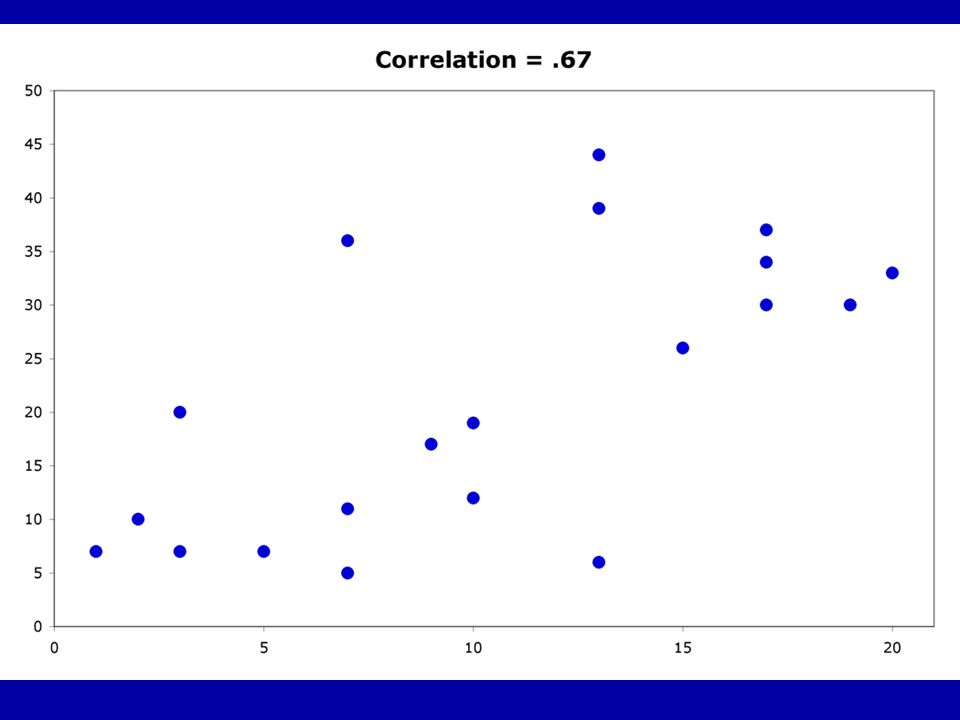
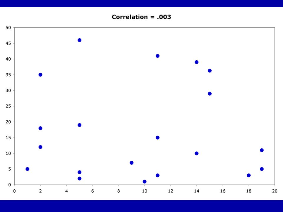
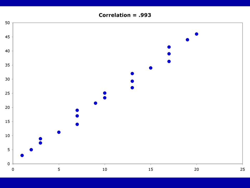
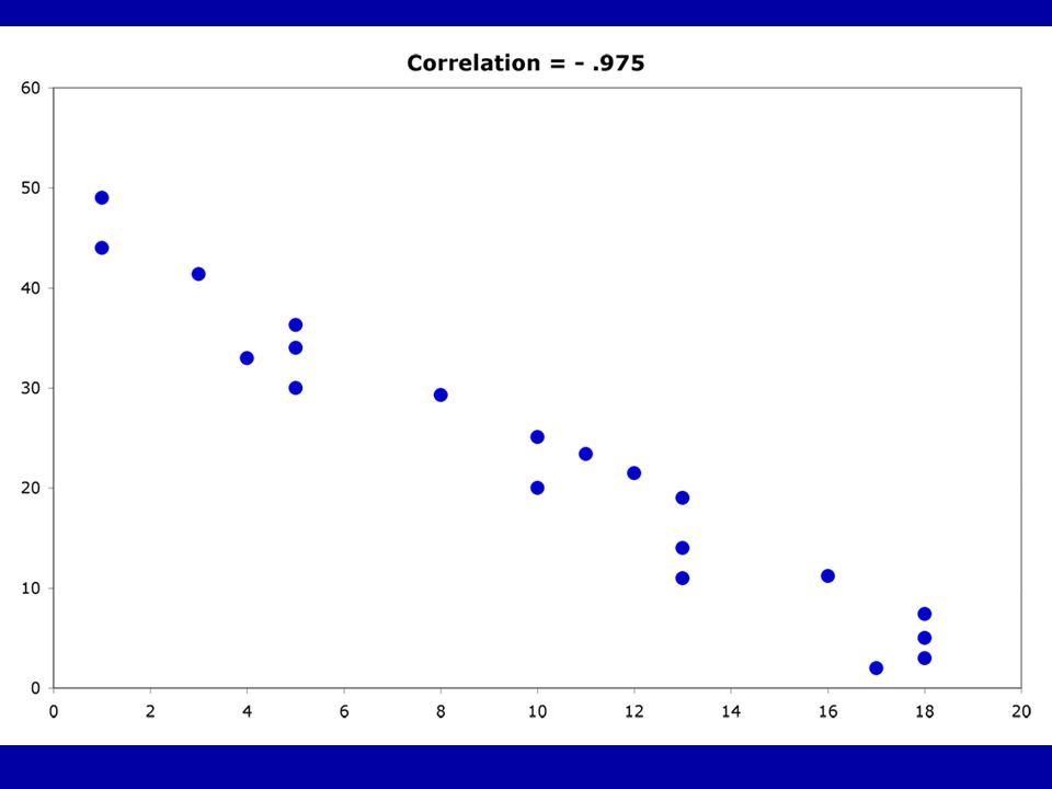
59. Guess the Correlations:.67.993.003 -.975

64.         []      [] The Pearson r r =

65.  Sum of the Xs   Sum of the Ys    Sum of the Xs squared  )   Sum of the Ys squared    Sum of the squared Xs    Sum of the squared Ys    Sum of Xs times the Ys   Number of Subjects  We Need:

66. Example: A sample of 6 children was selected, data about their age in years and weight in kilograms was recorded as shown in the following table. Find the correlation between age and weight. A sample of 6 children was selected, data about their age in years and weight in kilograms was recorded as shown in the following table. Find the correlation between age and weight. Weight (Kg) Age (years) serial No 1271 862 83 1054 1165 1396

67. Y2Y2 X2X2 xy Weight (Kg) (y) Age (years) (x) Serial n. 1444984127 1 64364886 2 1446496128 3 1002550105 4 1213666116 5 16981117139 6 ∑y2= 742 ∑x2= 291 ∑xy= 461 ∑y= 66 ∑x= 41 Total

68. r = 0.759 strong direct correlation

69. EXAMPLE: Relationship between Anxiety and Test Scores Anxiety(X) Test score (Y) X2X2X2X2 Y2Y2Y2Y2XY 102100420 8364924 2948118 171497 56253630 65362530 ∑X = 32 ∑Y = 32 ∑X 2 = 230 ∑Y 2 = 204 ∑XY=129

70. Calculating Correlation Coefficient r = - 0.94 Indirect strong correlation

71. a correlation coefficient (r) provides a quantitative way to express the degree of linear relationship between two variables. Range: r is always between -1 and 1 Sign of correlation indicates direction: - high with high and low with low -> positive - high with low and low with high -> negative - no consistent pattern -> near zero Magnitude (absolute value) indicates strength (-.9 is just as strong as.9).10 to.40 weak.40 to.80 moderate.80 to.99 high 1.00 perfect Correlation Coefficient

72. About “r”  r is not dependent on the units in the problem  r ignores the distinction between explanatory and response variables  r is not designed to measure the strength of relationships that are not approximately straight line  r can be strongly influenced by outliers

73. Correlation Coefficient: Limitations 1.Correlation coefficient is appropriate measure of relation only when relationship is linear 2.Correlation coefficient is appropriate measure of relation when equal ranges of scores in the sample and in the population. 3.Correlation doesn't imply causality –Using U.S. cities a cases, there is a strong positive correlation between the number of churches and the incidence of violent crime –Does this mean churches cause violent crime, or violent crime causes more churches to be built? –More likely, both related to population of city (3d variable -- lurking or confounding variable)

74. Ice-cream sales are strongly correlated with crime rates. Therefore, ice-cream causes crime.

75. Without proper interpretation, causation should not be assumed, or even implied.

76. In conclusion ! Z-test will be used for both categorical(qualitative) and quantitative outcome variables. Student’s t-test will be used for only quantitative outcome variables. Correlation will be used to quantify the linear relationship between two quantitative variables