1. Designing Optimal Taxes with a Microeconometric Model of Labour Supply Evidence from Norway Rolf Aaberge, Ugo Colombino and Tom Wennemo WPEG Conference, Canterbury, 11-13 July 2206

2. Purpose Identify optimal tax rules Use a microeconometric model of household labour supply Personal income taxes Norway

3. Standard approach empirical optimal taxation The typical exercise (e.g as surveyed by Tuomala): Take some optimal tax formula derived from theory Calibrate the parameters (preferences, distribution of characteristics etc.) using previous empirical results Compute optimal taxes

4. Standard approach in empirical optimal taxation Problem with this approach: theoretical results typically rely on some special assumptions possible inconsistency between the assumptions of the theoretical model and the assumptions of the empirical analysis used to calibrate the parameters

5. A “brute force” approach The approach adopted in this paper is radically different We do not start from a priori theoretical results We directly identify the optimal tax rule by running a microeconometric model of household labour supply that simulates household choices and utility for any tax rule The simulation searches for the tax rule that maximises a social welfare function subject to the constraint of a constant total tax revenue

6. The model We use a model of labour supply which features:model of labour supply simultaneous treatment of spouses’ decisions exact representation of complex tax rules quantity constraints on the choice of hours of work choice among jobs that differ with respect to hours, wage rate and other characteristics Separate models are estimated for couples and singles

7. The model max U(C, h, j ) s.t. C=f(wh, I) (h, w, j )  B U( ) = utility function f( ) = tax rule (turns gross incomes into net) C = net income h = labour supply w = wage rate I = exogenous income j = other job characteristics B = opportunity set

8. Basic assumptions U( f(wh,I), h, j) = V( f(wh,I), h) e(j) Prob(e < k) = exp(-1/k) = extreme value Type III p(w,h) = density of jobs of type (w,h) in Bdensity of jobs of type (w,h) in B

9. Choice probability... Then Prob((w,h) is chosen) = = V( f(wh,I),h)p(w,h) /  x,y V( f(xy,I), y)p(x,y)

10. Labour supply elasticities Labour supply elasticities implied by the model Married couples, Norway 1994

11. Simulating optimal tax rules STEP 1: Given a tax rule g( ), compute for each household i u i = max V( g(wh, I), h)e(j) s.t. (h, w, j)  B STEP 2: Compute the Social Welfare Function W(u 1,…,u N )Social Welfare Function u 1,…,u N STEP 3: Iterate (on the set of tax rules) STEPS 1-2 so as to maximize W keeping constant the total net tax revenueset of tax rules

12. Interpersonally comparable utility levels The arguments u i of the Social Welfare function are made interpersonally comparable by using a common utility function

13. Social Welfare Function Social Welfare Function (EO criterion) We use the class of the rank-dependent social welfare functions W. Let v(r) = utility level of the household at rank-position r Then W = ∑ r v(r) q(r, A) = (∑ r v(r) /N)(1 – G(A)) where q(r, A) is a weight that depends (1) on the rank-position r (2) on a parameter A that accounts for the social attitude towards inequality and G(A) is an inequality coefficient that depends on A. With different values of A we get different SW functions, e.g. Utilitarian, Gini, Bonferroni (in increasing order of inequality aversion).

14. Social Welfare Function Social Welfare Function (EOp criterion) The Equality-of-Opportunity (J. Roemer) criterion is a modification of the EO criterion. We partition the sample according to the value of exogenous variables that will be interpreted as measuring opportunities. We define: v(s,r) = utility level of the household at rank-position r in subsample s. Then the EOp W is W = ∑ r min s v(s,r) q(r, A)

15. 6-parameter piecewise linear tax rules The optimal tax rule is defined by 6 parameters: E = exemption level Z 1 = upper limit of first tax bracket Z 2 = upper limit of the second tax bracket t 1 = marginal rate of the first tax bracket t 2 = marginal rate of the second tax bracket t 3 = marginal rate of the third tax bracket It replaces the current 1994 rule, which is also piecewise linear, with seven income brackets and a smooth sequence of marginal rates (starting with.25 and ending up with.495). All transfers (social assistance, benefits etc.) are left unchanged.

16. Net GrossZ1Z1 Z2Z2 E t1t1 t2t2 t3t3

17. Net GrossZ1Z1 Z2Z2 E t1t1 t2t2 t3t3

18. Net Gross Z1Z1 Z2Z2 t1t1 t2t2

19. Optimal tax rules according to alternative social welfare criteria EO-social welfareEOp-social welfare BonferroniGiniUtilitarianBonferroniGiniUtilitarian t1t1 0.120.170.230.110.130.17 t2t2 0.380.350.320.410.370.31 t3t3 1.00 E2.0016.0020.002.000.00 Z1Z1 128.21141.42242.04130.22133.74147.55 Z2Z2 730.00720.00780.00740.00730.00710.00

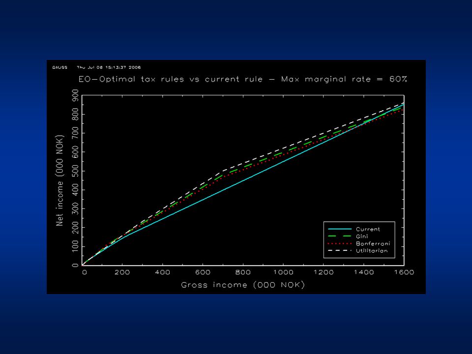
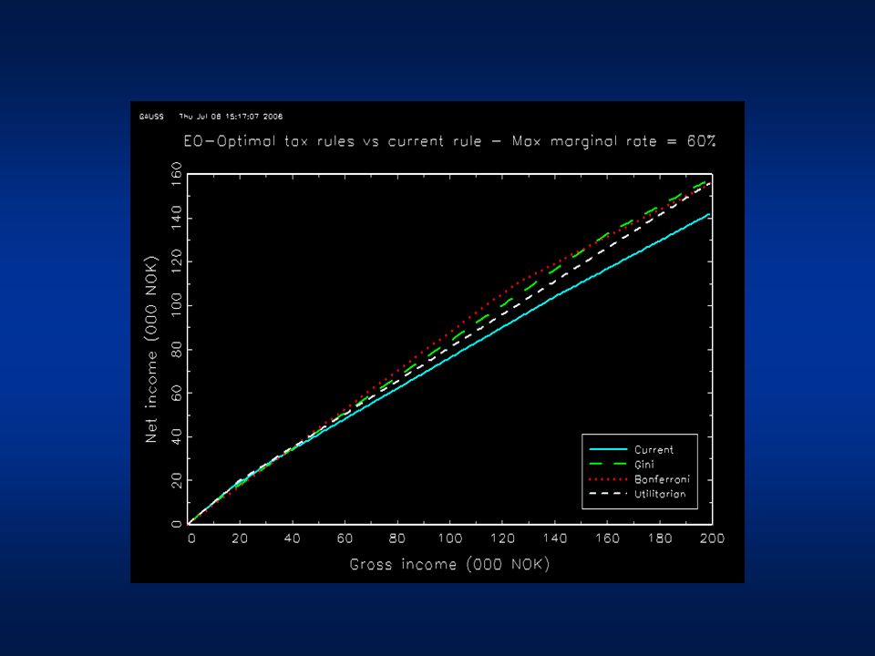
22. Optimal tax rules according to alternative social welfare criteria Maximum marginal rate = 60% EO-social welfareEOp-social welfare BonferroniGiniUtilitarianBonferroniGiniUtilitarian t1t1 0.120.180.240.120.140.17 t2t2 0.380.360.330.410.370.31 t3t3 0.60 E0.001.0020.001.000.00 Z1Z1 124.75159.43288.69132.68136.04137.63 Z2Z2 700.00

25. Percentage variation in labour supply when the EO-GINI- optimal tax rule is applied (t 3 constrained to be 0.6)labour supply Household Income Decile Single male Single female Married male Married female I64.2365.8731.4740.78 II16.7311.3122.1711.42 III - VIII1.821.063.302.76 IX0.00 1.81-1.23 X0.00 -2.64-0.57

26. Comments Similar to the current rule, optimal tax rules imply a sequence of increasing marginal tax rates However, optimal rules are much more progressive on high income levels and much less progressive on low and average income levels (somehow consistent with the pattern of labour supply elasticities)labour supply elasticities Optimal rules imply a higher net income for almost any level of gross income (except for very high incomes)  lower average tax rate: thanks to a sufficiently large labour supply responselabour supply response

27. References Aaberge, R.., J.K. Dagsvik and S. Strøm (1995): "Labor Supply Responses and Welfare Effects of Tax Reforms", Scandinavian Journal of Economics, 97, 4, 635-659. Aaberge, R., U. Colombino and S. Strøm (1999): “Labor Supply in Italy: An Empirical Analysis of Joint Household Decisions, with Taxes and Quantity Constraints”, Journal of Applied Econometrics, 14, 403-422. Aaberge, R., U. Colombino and S. Strøm (2000): “Labour supply responses and welfare effects from replacing current tax rules by a flat tax: empirical evidence from Italy, Norway and Sweden”, Journal of Population Economics, 13, 595-621. Aaberge, R., U. Colombino and S. Strøm (2004): "Do More Equal Slices Shrink the Cake? An Empirical Investigation of Tax- Transfer Reform Proposals in Italy“, Journal of Population Economics, 17

28. The opportunity set The opportunity set (illustrative example) 20 80 5 h w 0 40 2 20 30 3