1. Inference for  0 and 1 Confidence intervals and hypothesis tests

2. Example 1: Relation between leg strength and punting distance? PUNTER LEG DIST 1 170 162.50 2 140 144.00 3 180 147.50 4 160 163.50 5 170 192.00 6 150 171.75 7 170 162.00 8 110 104.83 9 120 105.67 10 130 117.58 11 120 140.25 12 140 150.16 13 160 165.16 13 punters in American football DIST = average length (feet) of 10 punts LEG = strength of leg (pounds lifted)

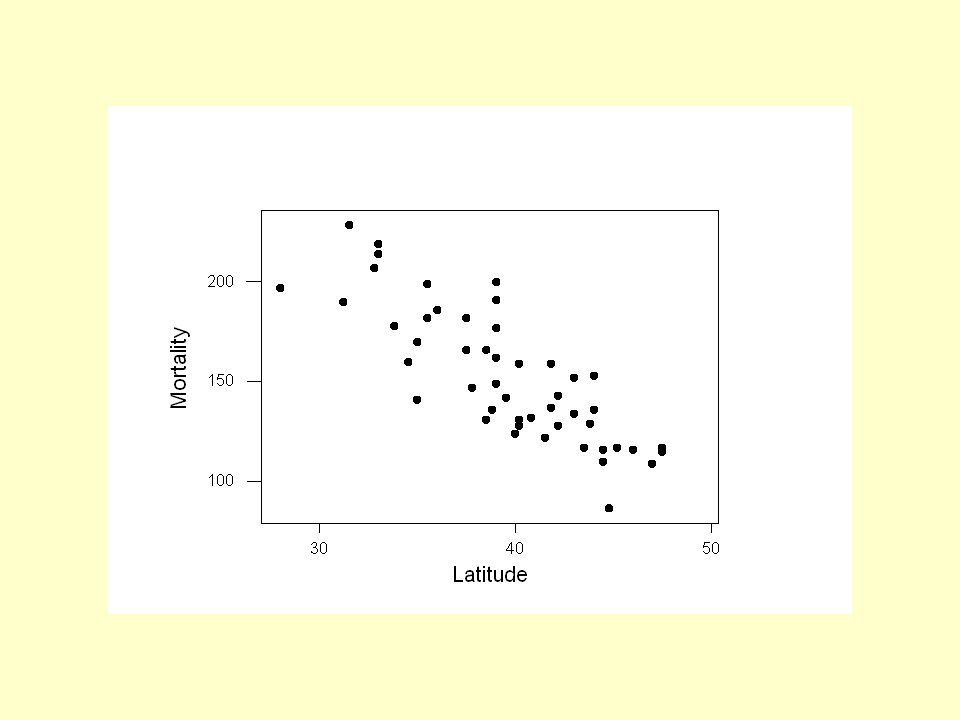
3. Example 2: Relation between state latitude and skin cancer mortality? # State LAT MORT 1 Alabama 33.0 219 2 Arizona 34.5 160 3 Arkansas 35.0 170 4 California 37.5 182 5 Colorado 39.0 149 !    49 Wyoming 43.0 134 Mortality rate of white males due to malignant skin melanoma from 1950-1959. LAT = degrees (north) latitude of center of state MORT = mortality rate due to malignant skin melanoma per 10 million people

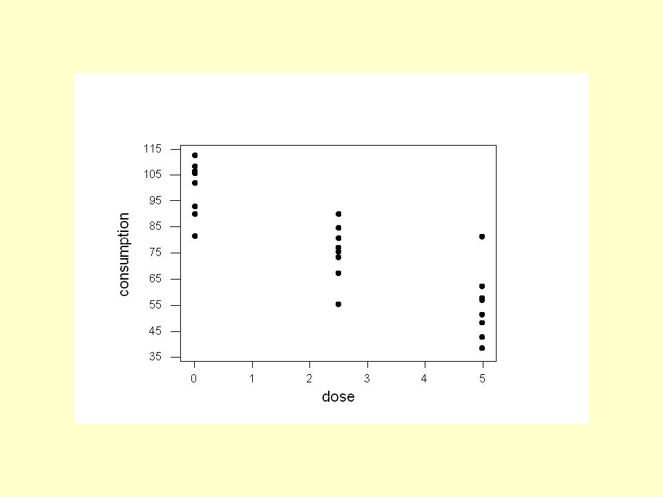
4. Example 3: Relation between use of amphetamines and food consumption? X = Amphetamine dose (mg/kg) 0 2.5 5.0 112.6 73.3 38.5 102.1 84.8 81.3 90.2 67.3 57.1 81.5 55.3 62.3 105.6 80.7 51.5 93.0 90.0 48.3 106.6 75.5 42.7 108.3 77.1 57.9 24 rats randomly allocated to dose of amphetamine (saline (0), 2.5, and 5.0 mg/kg) Y = amount of food (grams of food consumed per kilogram of body weight) in following 3-hour period

5. Point estimates b 0 and b 1 The b 0 and b 1 values vary. They depend on the particular (x i, y i ) sample obtained.

6. Assumptions about error terms  i E(  i ) = 0  i and  j are uncorrelated Var(  i ) =  2 (New!!)  i are normally distributed NOTE: All results thus far (such as least squares estimates, Gauss-Markov Theorem, and mean square error) only depend on first three assumptions. Today’s results depend on normality of the error terms.

7. Sampling distribution of b 1 b 1 is normally distributed Providing error terms  i are normally distributed: with mean 1 and variance

8. Recall: Confidence interval for  using  Sample estimate ± margin of error

9. Confidence interval for 1 using b 1 Sample estimate ± margin of error

10. Recall: Hypothesis testing for  using  The null (H 0 :  =  0 ) versus the alternative (H A :  ≠  0 ) Test statistic P-value = How likely is it that we’d get a test statistic t* as extreme as we did if the null hypothesis is true? The P-value is determined by comparing the test statistic t* to a t-distribution with n-1 degrees of freedom.

11. Hypothesis testing for 1 using b 1 The null (H 0 : 1 = ) versus the alternative (H A : 1 ≠ ) Test statistic P-value = How likely is it that we’d get a test statistic t* as extreme as we did if the null hypothesis is true? The P-value is determined by comparing the test statistic t* to a t-distribution with n-2 degrees of freedom.

12. Sampling distribution of b 0 b 0 is normally distributed Providing error terms  i are normally distributed: with mean 0 and variance

13. Confidence interval for 0 using b 0 Sample estimate ± margin of error

14. Hypothesis testing for 0 using b 0 The null (H 0 : 0 = ) versus the alternative (H A : 0 ≠ ) Test statistic P-value = How likely is it that we’d get a test statistic t* as extreme as we did if the null hypothesis is true? The P-value is determined by comparing the test statistic t* to a t-distribution with n-2 degrees of freedom.

17. Example 1: Inference The regression equation is punt = 14.9 + 0.903 leg Predictor Coef SE Coef T P Constant 14.91 31.37 0.48 0.644 leg 0.9027 0.2101 4.30 0.001 S = 16.58 R-Sq = 62.7% R-Sq(adj) = 59.3% Unusual Observations Obs leg punt Fit SE Fit Residual St Resid 3 180 147.50 177.39 8.20 -29.89 -2.07R R denotes an observation with a large standardized residual

20. Example 2: Inference The regression equation is Mortality = 389 - 5.98 Latitude Predictor Coef SE Coef T P Constant 389.19 23.81 16.34 0.000 Latitude -5.9776 0.5984 -9.99 0.000 S = 19.12 R-Sq = 68.0% R-Sq(adj) = 67.3% Unusual Observations Obs Latitude Mortality Fit SE Fit Residual St Resid 7 39.0 200.00 156.06 2.75 43.94 2.32R 9 28.0 197.00 221.82 7.42 -24.82 -1.41 X 30 35.0 141.00 179.97 3.85 -38.97 -2.08R R denotes an observation with a large standardized residual X denotes an observation whose X value gives it large influence.

23. Example 3: Inference The regression equation is consumption = 99.3 - 9.01 dose Predictor Coef SE Coef T P Constant 99.331 3.680 26.99 0.000 dose -9.008 1.140 -7.90 0.000 S = 11.40 R-Sq = 73.9% R-Sq(adj) = 72.8% Unusual Observations Obs dose consumpt Fit SE Fit Residual St Resid 18 5.00 81.30 54.29 3.68 27.01 2.50R R denotes an observation with a large standardized residual.

24. Inference for 0 and 1 in Minitab Select Stat. Select Regression. Select Regression … Specify Response (y) and Predictor (x). Click on OK.