Download presentation
Presentation is loading. Please wait.

1
Sampling Distributions Statistics 2126

2
Introduction Let’s assume that the IQ in the population has a mean ( ) of 100 and a standard deviation ( ) of 15 In fact the tests are designed that way so we are in luck, we know the parameters
 of 100 and a standard deviation ( ) of 15 In fact the tests are designed that way so we are in luck, we know the parameters")
3
A Little Thought experiment Let’s randomly select 20 people and measure their IQs Let’s calculate the mean for each group sampled What would you expect to get? What would you really get? What would the curve look like?

5
Another thought experiment Assigning the value of 0 to women and 1 to men for the variable ‘maleness’ Let’s select 20 adults, randomly What value should we get for maleness What value would we get What would the curve look like?

7
No way.. Way… Think about it You will get, usually, the same number of males and females Sometimes very few of either

8
Sampling Distributions These two distributions are called sampling distributions In this case, the sampling distribution of the mean All the possible values a statistic can take with a given sample size

9
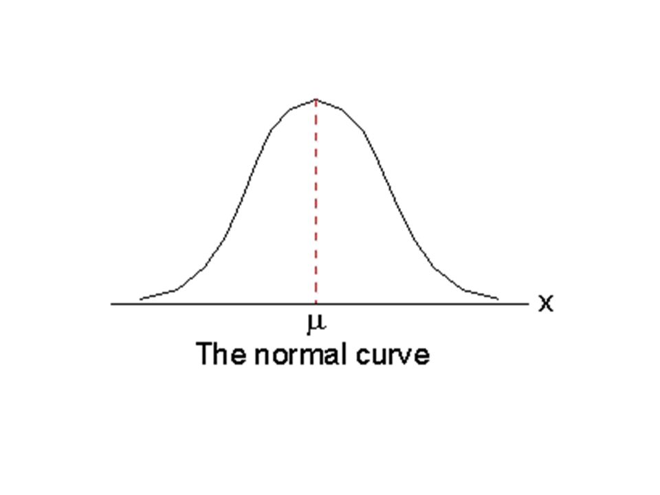
The Central Limit Theorem Given a population distribution with a mean ( ) and a standard deviation ( ) the sampling distribution of the mean will have a mean = and a variance of 2 /n and will approach normal as n increases no matter what the shape of the parent population distribution
 and a standard deviation ( ) the sampling distribution of the mean will have a mean = and a variance of 2 /n and will approach normal as n increases no matter what the shape of the parent population distribution")
10
Pretty cool So now we can combine this knowledge with what we know about the z distribution and figure out how likely a given mean is Well we know the shape, the mean and the standard deviation so now finding the likelihood of a given mean for a variable is the same as doing it for a given value

11
Whaaaa? Well before we could find out how likely an IQ of 108 was. OK, so let’s do that with a mean of 108 n = 9 It is IQ so = 100 And = 15

12
Do the plusses and takeaways… z = (x- ) / But we have a sampling distribution so z = ( - ) / ( / n) z = (108-100) / (15/3) z = 8 / 5 z = 1.6 p(z > 1.6) =.055
 / But we have a sampling distribution so z = ( - ) / ( / n) z = ( ) / (15/3) z = 8 / 5 z = 1.6 p(z > 1.6) =.055")
13
So how can we use this knowledge? Say you flip a coin At some point you say well that is a fixed coin, not a fair coin But at what level? Well when the probability that it is a fair coin in < some value (usually.05)
.")
14
Hypotheses We set up two, mutually exclusive hypotheses H 0 and H A The null is that there is no effect The alternative is that there is an effect If the p(H 0 is true) <.05 the we reject H 0
 <.05 the we reject H 0")
15
So in our example p(z > 1.6) =.055 Darn, too high We fail to reject H 0 Not enough evidence Pretty darned close though
 =.055 Darn, too high We fail to reject H 0 Not enough evidence Pretty darned close though")
16
Now we can make mistakes False positives False negatives

17
Errors in hypothesis testing Reality Decision H 0 trueH a true Do not reject H 0 Correct decision Type II error Reject H 0 Type I errorCorrect decision

Similar presentations


>")


2000 South-Western College.>")