1. Chapter 22 Comparing Two Proportions

2.  Comparisons between two percentages are much more common than questions about isolated percentages.  We often want to know how two groups differ, whether a treatment is better than a placebo control, or whether this year’s results are better than last year’s.

3. The Standard Deviation of the Difference Between Two Proportions  Proportions observed in independent random samples are independent. Thus, we can add their variances. So…  The standard deviation of the difference between two sample proportions is  Thus, the standard error is

4. Assumptions and Conditions  Independence Assumptions: –Randomization Condition: The data in each group should be drawn independently and at random from a homogeneous population or generated by a randomized comparative experiment. –The 10% Condition: If the data are sampled without replacement, the sample should not exceed 10% of the population. –Independent Groups Assumption: The two groups we’re comparing must be independent of each other.

5. Assumptions and Conditions (cont.)  Sample Size Condition: –Each of the groups must be big enough… –Success/Failure Condition: Both groups are big enough that at least 10 successes and at least 10 failures have been observed in each.

6. The Sampling Distribution  We already know that for large enough samples, each of our proportions has an approximately Normal sampling distribution.  The same is true of their difference.

7. The Sampling Distribution (cont.)  Provided that the sampled values are independent, the samples are independent, and the samples sizes are large enough, the sampling distribution of is modeled by a Normal model with –Mean: –Standard deviation:

8. Two-Proportion z-Interval  When the conditions are met, we are ready to find the confidence interval for the difference of two proportions:  The confidence interval is where  The critical value z* depends on the particular confidence level, C, that you specify.

9. Everyone into the Pool  The typical hypothesis test for the difference in two proportions is the one of no difference. In symbols, H 0 : p 1 – p 2 = 0.  Since we are hypothesizing that there is no difference between the two proportions, that means that the standard deviations for each proportion are the same.  Since this is the case, we combine (pool) the counts to get one overall proportion.

10. Everyone into the Pool (cont.)  The pooled proportion is where and –If the numbers of successes are not whole numbers, round them first. (This is the only time you should round values in the middle of a calculation.)

11. Everyone into the Pool (cont.)  We then put this pooled value into the formula, substituting it for both sample proportions in the standard error formula:

12. Two-Proportion z-Test  The conditions for the two-proportion z-test are the same as for the two-proportion z-interval.  We are testing the hypothesis H 0 : p 1 = p 2.  Because we hypothesize that the proportions are equal, we pool them to find

13. Two-Proportion z-Test (cont.)  We use the pooled value to estimate the standard error:  Now we find the test statistic:  When the conditions are met this statistic follows the standard Normal model, so we can use that model to obtain a P-value.

14. EXAMPLE Would being a part of a support group that meets regularly help people who are wearing the nicotine patch actually quit smoking? Volunteer subjects are randomly divided into two groups. Group 1 members were given the patch and attended a weekly discussion meeting. Group 2 members also used the patch but did not participate in the meetings. After six months 46 of the 143 in Group 1 and 30 of 151 smokers in Group 2 had successfully stopped smoking. Do these results suggest that support groups could be an effective way to help people stop smoking?

15. 1. Hypotheses 2. Model

16. 1. Hypotheses 2. Model  2-proportion z-test  Randomization  10% Condition  At least 10 success and 10 failures for both groups Since all conditions are satisfied, use the normal model to approximate p 2 = proportion of Group 2 members who quit p 1 = proportion of Group 1 members who quit

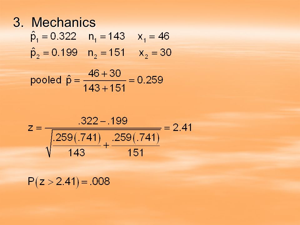
17. 3. Mechanics

19. 4. Conclusion Because our p-value of 0.008 is less than.05 (alpha), we reject the null hypothesis that claims that the same proportion of people quit smoking regardless of whether they go to a weekly support meeting.

20. What Can Go Wrong?  Don’t use two-sample proportion methods when the samples aren’t independent. –These methods give wrong answers when the independence assumption is violated.  Don’t apply inference methods when there was no randomization. –Our data must come from representative random samples or from a properly randomized experiment.  Don’t interpret a significant difference in proportions causally.