1. The ENSEMBLES high- resolution gridded daily observed dataset Malcolm Haylock, Phil Jones, Climatic Research Unit, UK WP5.1 team: KNMI, MeteoSwiss, Oxford University

2. Outline The gridded dataset: who, why, when and what? The station network Interpolation –method comparison –two-step interpolation of monthly and daily data –kriging and extremes Point vs interpolated extremes –implication for RCM validation Uncertainty Then finally some analyses comparing with GCM simulations from RT2B with ERA-40 forcing

3. The dataset… Who: –Four groups in WP5.1 –KNMI: data gathering and data quality and homogenisation –MeteoSwiss: homogeneity of temperature data –UEA and Oxford: interpolation Why –Validation of RCMs –Climate change studies –Impacts models –Many data providers do not allow distribution of station data

4. …The dataset… When –Daily 1950-2006 –Available now from ENSEMBLES web site plus ECA&D –Two papers submitted to JGR, one on the comparison of methods, and one on the final gridded dataset with the chosen methods, which differ by variable What –Five variables precipitation mean, minimum and maximum temperature mean sea level pressure (early 2008) – Europe 0.25 0 and 0.5 0 CRU grids common RCM rotated-pole grid 0.22 0 and 0.44 0 rotated pole (-162.0 0, 39.25 0 )

5. No. of stations

6. Precipitation Stations 2050

7. Tmean Stations 1231

8. Interpolation Need to match observations to model grid for direct comparison Therefore need to estimate observations at “unsampled” locations Compare several methods to find most accurate at reproducing observations in a cross validation exercise – see more in Nynke Hofstra’s presentation tomorrow Largest QC problem is that date of observations do not match – day is day when values occurred, but sometimes it is day when measured

9. Interpolation Methods Natural neighbour interpolation Angular distance weighting Thin-plate splines –2-D and 3-D Kriging –2-D and 3-D 4-D Regression –lat, lon, elevation and distance to coast Conditional Interpolation – important for precipitation

10. Stochastic or Deterministic Stochastic –assumes that an interpolated surface is just one of many, all of which could produce the observations –models the data with a statistical distribution to determine the expected mean at unsampled locations –probabilistic model allows uncertainty estimates Deterministic –assumes only one possible interpolated surface –adopts a particular geographical model e.g. bilinear, inverse distance, Thiessen polygons

11. Cross Validation. For each station, interpolate to that station using its neighbours and compare with the observed value. –Repeat for all days. –Do for monthly averages and daily anomalies Daily precipitation (% of monthly total) compound relative error (cre) = rms / σ critical success index (csi) = hits/(false alarm+hits+misses)

12. Cross Validation Daily pressure (anomaly from monthly mean) Daily Tmean (anomaly from monthly mean) precip: 2-D kriging with separate occurrence model pressure: 2-D kriging Tmean, Tmin, Tmax: 3-D kriging

13. Interpolation methodology Grid monthly means using 2-D (pressure) and 3-D (temp and precipitation) thin-plate splines –Determined to be the best method using cross validation Grid daily anomalies using kriging Combine the interpolated monthly means and the interpolated anomalies as well as their uncertainty Create a high resolution master grid (10km rotated-pole grid) and do area averaging to create different coarser resolution products.

14. Kriging and extremes Kriging estimates the mean and variance of the distribution at unsampled locations The best guess is the mean but extremes are usually a combination of a high local signal superimposed on a high background state Therefore kriging will tend to underestimate extremes and produce results similar to the area mean

15. Precipitation interpolation extremes reduction factor 50% 75% 90% 95% 99% 2yr 5yr 10yr

16. Tmax interpolation extremes - reduction in anomaly 50%75% 90% 95% 99% 2yr 5yr 10y r

17. Gridded Extremes precipitation 10-year return period Extremes of Gridded Precipitation Extremes

18. Uncertainty Interpolation uncertainty only

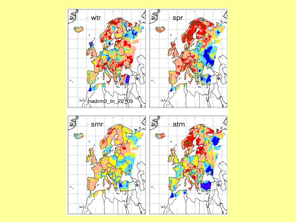
20. Conclusions We have created a European daily dataset very much improved over previous products, with a detailed comparison of interpolation methods Kriging gives the best estimate of a point source, but when the interpolated grid (25km) is smaller than the average separation (45km for precipitation), the interpolated point will be more an area average Therefore validation of RCMs using the gridded data assumes the RCMs represent area-averages Kriging can be extended to produce more realistic “simulations” of point precipitation at unsampled locations, with a better estimate of uncertainty of the extremes, but this is computationally very expensive

21. ENSEMBLES WP5.4 and ETCCDI Meeting – KNMI De Bilt – 13-16 May 2008 Extremes of temperature and precipitation as seen in the daily gridded datasets for surface climate variables (D5.18 – Haylock et al.) and in the RCM model output from the (RT3) 40-year experiments driven by ERA-40 reanalysis data Phil Jones and David Lister – Climatic Research Unit

22. Gridded Data Available on ENSEMBLES web site Two papers submitted to JGR One on a comparison of gridding techniques (Hofstra et al.) One on the final gridded dataset (Haylock et al.) A simple comparison shown here

23. The location and period of coverage of station-series which went into the interpolation/gridding exercise

24. Extreme Measures Trends of mean maximum and minimum temperatures Trends of 5 th percentile of Tn Trends of 95 th percentile of Tx Compare gridded trends with station trends Trends patterns over various periods

25. Testing of extreme values in a fairly flat part of the region covered by the observed grids – Lubny, Ukraine

26. As earlier, but JJA

27. Trends (°C/decade) in the (gridded/observed) 05 th percentile Tmin. series – 1950-2006

28. Trends (°C/decade) in the CRU 0.5° grids (CRU TS3.0) Tmin. series – 1950-2006

29. Trends (°C/decade) in the (gridded/observed) 95 th percentile Tmax. series – 1950-2006

30. Trends (°C/decade) in the (gridded/observed) 05 th percentile Tmin. series – 1961-2006

31. Trends (°C/decade) in the (gridded/observed) 95 th percentile Tmax. series – 1961-2006

32. Tn05 – histogram of differences compared to gridded observations

33. Tx95 – histogram of differences compared to gridded observations