1. Statistical Models for Automatic Speech Recognition Lukáš Burget

2. Feature extraction Preprocessing speech signal to satisfy needs of the following recognition process (dimensionality reduction, preserving only the “important” information, decorelation). Popular features are MFCC: modification based on psycho-acoustic findings applied to short-time spectra. For convenience, we will use one-dimensional features in most of our examples (e.g. short time energy).

3. Classifying single speech frame unvoicedvoiced

4. Classifying single speech frame unvoicedvoiced Mathematically, we ask the following question: But the value we read from probability distribution is p(x|class ). p ( x j vo i ce d ) P ( vo i ce d ) p ( x ) > p ( x j unvo i ce d ) P ( unvo i ce d ) p ( x ) P ( vo i ce d j x ) > P ( unvo i ce d j x ) According to Bayes Rule, the above can be revritten as:

5. Multi-class classification unvoicedvoicedsilence The class being correct with the highest probability is given by: argmax ! P ( ! j x ) = argmax ! p ( x j ! ) P ( ! ) But we do not know the true distribution, …

6. Estimation of parameters unvoicedvoicedsilence … we only see some training examples.

7. Estimation of parameters unvoicedvoicedsilence … we only see some training examples. Let’s decide for some parametric model (e.g. Gaussian distribution) and estimate its parameters from the data.

8. Maximum Likelihood Estimation In the next part, we will use ML estimation of model parameters: This allow as to individually estimate parameters, Θ, of each class given the data for that class. Therefore, for the convenience, we can omit the class identities in the following equations. The models we are going to examine are: –Single Gaussian –Gaussian Mixture Model (GMM) –Hidden Markov Model We want to solve three fundamental problems: –Evaluation of the model (computing likelihood of features given the model) –Training the model (finding ML estimates of parameters) –Finding most likely values of hidden parameters ^ £ c l ass ML = argmax £ Y 8 x i 2 c l ass p ( x i j £ )

9. Gaussian distribution (1 dimension) N ( x;¹ ; ¾ 2 ) = 1 ¾ p 2 ¼ e ¡ ( x ¡ ¹ ) 2 2 ¾ 2 ¹ = 1 T P T t = 1 x ( t ) ML estimates of parameters (Training): ¾ 2 = 1 T P T t = 1 ( x ( t ) ¡ ¹ ) 2 Evaluation: No hidden variables.

10. Gaussian distribution (2 dimensions) N ( x ; ¹ ; § ) = 1 p ( 2 ¼ ) P j § j e ¡ 1 2 ( x ¡ ¹ ) T § ¡ 1 ( x ¡ ¹ )

11. Gaussian Mixture Model p ( x j £ ) = P c P c N ( x;¹ c ; ¾ 2 c ) Evaluation: where P c P c = 1

12. Gaussian Mixture Model p ( x j £ ) = P c P c N ( x;¹ c ; ¾ 2 c ) Evaluation: We can see the sum above just as a function defining the shape of the probability density function, or we can see it as a more complicated generative probabilistic model, from which features are generated as follows: – One of Gaussian components is first randomly selected according prior probabilities Pc –Feature vector is generated form the selected Gaussian distribution For the evaluation, however, we do not know which component generated the input vector (Identity of the component is hidden variable). Therefore, we marginalize – sum over all the components respecting their prior probabilities. Why we want to complicate our lives with this concept: –It allows at to apply EM algorithm for GMM training –We will need this concept for HMMs

13. Training GMM –Viterbi training Intuitive and Approximate iterative algorithm for training GMM parameters. Using current model parameters, let Gaussians to classify data as the Gaussians were different classes (Even though the both data and all components corresponds to one class modeled by the GMM) Re-estimate parameters of Gaussian using the data associated with to them in the previous step. Repeat the previous two steps until the algorithm converge.

14. Training GMM – EM algorithm ^ ¹ ( new ) c = P T t = 1 ° c ( t ) x ( t ) P T t = 1 ° c ( t ) ^ ¾ 2 c ( new ) = P T t = 1 ° c ( t )( x ( t ) ¡ ^ ¹ ( new ) c ) 2 P T t = 1 ° c ( t ) ° c ( t ) = P c N ( x ( t ) ; ^ ¹ ( o ld ) c ; ^ ¾ 2 c ( o ld ) ) P c P c N ( x ( t ) ; ^ ¹ ( o ld ) c ; ^ ¾ 2 c ( o ld ) ) Expectation Maximization is very general tool applicable in many cases were we deal with unobserved (hidden) data. Here, we only see the result of its application to the problem of re- estimating parameters of GMM. It guarantees to increase likelihood of training data in every iteration, however it does not guarantees to find the global optimum. The algorithm is very similar to Viterbi training presented above. Only instead of hard decisions, it uses “soft” posterior probabilities of Gaussians (given the old model) as a weights and weight average is used to compute new mean and variance estimates.

16. unvoicedvoicedsilence Classifying stationary sequence P ( X j c l ass ) = Y 8 x i 2 c l ass p ( x i j c l ass ) Frame independency assumption

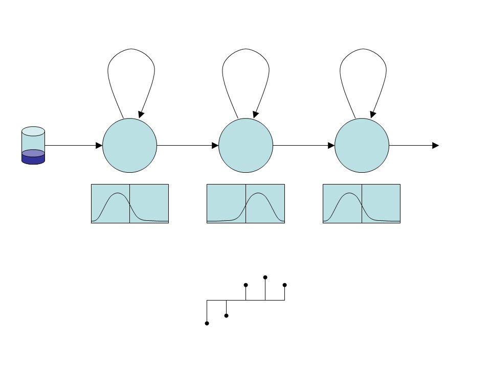
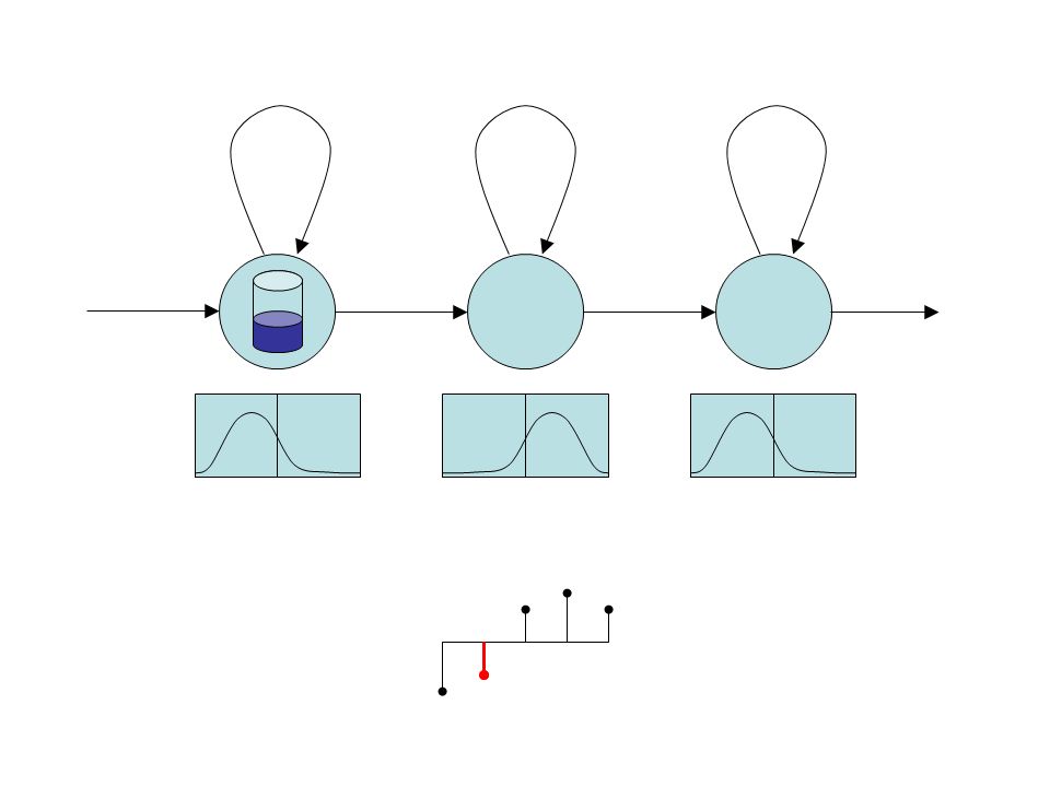
17. Modeling more general sequences: Hidden Markov Models a 11 a 22 a 33 a 12 a 34 a 23 b 1 (x)b 2 (x)b 3 (x) Generative model: For each frame, model moves from one state to another according to a transition probability a ij and generates feature vector from probability distribution b j (.) associated with the state that was entered. To evaluate such model, we do not see which path through the states was taken. Let’s start with evaluating HMM for a particular state sequence.

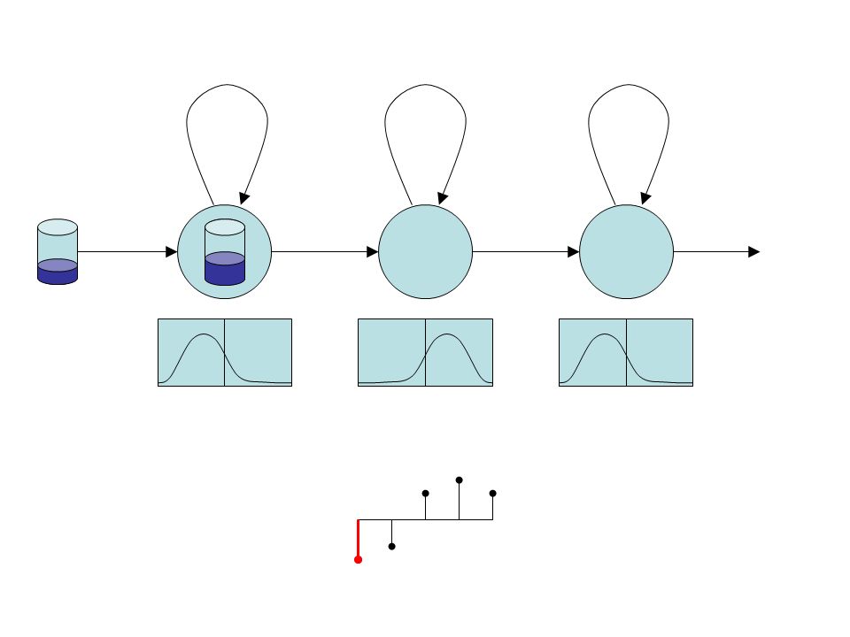
18. a 11 a 22 a 33 a 12 a 34 a 23 b 1 (x)b 2 (x)b 3 (x) a 11 a 12 a 23 a 33 P(X,S|Θ) = b 1 (x 1 ) b 1 (x 2 ) b 2 (x 3 ) b 3 (x 4 ) b 3 (x 5 )a 11 a 12 a 23 a 33 b 1 (x 1 ) b 1 (x 2 ) b 2 (x 3 ) b 3 (x 4 ) b 3 (x 5 )

19. a 11 a 12 a 23 a 33 P(X,S|Θ) = b 1 (x 1 ) b 1 (x 2 ) b 2 (x 3 ) b 3 (x 4 ) b 3 (x 5 )a 11 a 12 a 23 a 33 b 1 (x 1 ) b 1 (x 2 ) b 2 (x 3 ) b 3 (x 4 ) b 3 (x 5 ) Evaluating HMM for a particular state sequence

20. P ( X j S ; £ ) = b 1 ( x 1 ) b 1 ( x 2 ) b 2 ( x 3 ) b 3 ( x 4 ) b 3 ( x 5 ) P ( S j £ ) = a 11 a 12 a 23 a 33 a 34 P ( X ; S j £ ) = P ( X j S ; £ ) P ( S ; £ ) P ( X ; S j £ ) = b 1 ( x 1 ) a 11 b 1 ( x 2 ) a 12 b 2 ( x 3 ) a 23 b 3 ( x 4 ) a 33 b 3 ( x 5 ) a 34 where is prior probability of hidden variable – state sequence S. For GMM, the corresponding term was: P c is likelihood of observed sequence X, given the state sequence S. For GMM, the corresponding term was: N ( x ;¹ c ; ¾ 2 c ) The joint likelihood of observes sequence X and state sequence S can be decomposed as follows:

24. .

25. .

26. .

27. P ( X j £ ) = P S P ( X ; S j £ ) Evaluating HMM (for any state sequence) Since we do not know the underlying state sequence, we must marginalize – compute and sum likelihoods over all the possible paths

33. P ( X j £ ) = max S P ( X ; S j £ ) Finding the best (Viterbi) paths

34. Training HMMs – Viterbi training Similar to the approximate training we have already seen for GMMs 1.For each training utterance find Viterbi path through GMM, which associate feature frames with states. 2.Re-estimate state distribution using associated feature frames. 3.Repeat steps 1. and 2. until the algorithm converges.

35. Training HMMs using EM ^ ¹ ( new ) s = P T t = 1 ° s ( t ) x ( t ) P T t = 1 ° s ( t ) ^ ¾ 2 s ( new ) = P T t = 1 ° s ( t )( x ( t ) ¡ ^ ¹ ( new ) s ) 2 P T t = 1 ° s ( t ) ® s ( t ) ¯ s ( t ) t s ° s ( t ) = ® s ( t ) ¯ s ( t ) P ( X j £ ( o ld ) )

36. Isolated word recognition YES NO p ( X j YES ) P ( YES ) > p ( X j NO ) P ( NO )

37. YES NO sil Connected word recognition

38. Phoneme based models y eh s y s

39. w ah n t uw th r iy one two three sil P(one) P(three) P(two) Using Language model - unigram

40. ah n sil uw sil riy sil one two three w t th P(W 2 |W 1 ) one three two Using Language model - bigram

41. Other basic ASR topics not covered by this presentation Context dependent models Training phoneme based models Feature extraction –Delta parameters –De-correlation of features Full-covariance vs. diagonal cov. modeling Adaptation to speaker or acoustic condition Language Modeling –LM smoothing (back-off) Discriminative training (MMI or MPE) and so on