1. The Examination of Residuals

2. The residuals are defined as the n differences : where is an observation and is the corresponding fitted value obtained by use of the fitted model.

3. Many of the statistical procedures used in linear and nonlinear regression analysis are based certain assumptions about the random departures from the proposed model. Namely; the random departures are assumed i) to have zero mean, ii) to have a constant variance,  2, iii) independent, and iv) follow a normal distribution.

4. Thus if the fitted model is correct, the residuals should exhibit tendencies that tend to confirm the above assumptions, or at least, should not exhibit a denial of the assumptions.

5. The principal ways of plotting the residuals e i are: 1. Overall. 3. Against the fitted values 2. In time sequence, if the order is known. 4. Against the independent variables x ij for each value of j In addition to these basic plots, the residuals should also be plotted 5. In any way that is sensible for the particular problem under consideration,

6. Overall Plot The residuals can be plotted in an overall plot in several ways.

7. 1.The scatter plot. 2.The histogram. 3.The box-whisker plot. 4.The kernel density plot 5.a normal plot or a half normal plot on standard probability paper.

8. 2.The Chi-square goodness of fit test The standard statistical test for testing Normality are: 1.The Kolmogorov-Smirnov test.

9. The empirical distribution function is defined below for n random observations The Kolmogorov-Smirnov test The Kolmogorov-Smirnov uses the empirical cumulative distribution function as a tool for testing the goodness of fit of a distribution. F n (x) = the proportion of observations in the sample that are less than or equal to x.

10. Let F 0 (x) denote the hypothesized cumulative distribution function of the population (Normal population if we were testing normality) If F 0 (x) truly represented distribution of observations in the population than F n (x) will be close to F 0 (x) for all values of x.

11. The Kolmogorov-Smirinov test statistic is : = the maximum distance between F n (x) and F 0 (x). If F 0 (x) does not provide a good fit to the distributions of the observation - D n will be large. Critical values for are given in many texts

12. Let f i denote the observed frequency in each of the class intervals of the histogram. The Chi-square goodness of fit test The Chi-square test uses the histogram as a tool for testing the goodness of fit of a distribution. Let E i denote the expected number of observation in each class interval assuming the hypothesized distribution.

13. m = the number of class intervals used for constructing the histogram). The hypothesized distribution is rejected if the statistic: is large. (greater than the critical value from the chi-square distribution with m - 1 degrees of freedom.

14. Note. The in the above tests it is assumed that the residuals are independent with a common variance of  2. This is not completely accurate for this reason: Although the theoretical random errors  i are all assumed to be independent with the same variance  2, the residuals are not independent and they also do not have the same variance.

15. They will however be approximately independent with common variance if the sample size is large relative to the number of parameters in the model. It is important to keep this in mind when judging residuals when the number of observations is close to the number of parameters in the model.

16. Time Sequence Plot The residuals should exhibit a pattern of independence. If the data was collected in time there could be a strong possibility that the random departures from the model are autocorrelated.

17. Namely the random departures for observations that were taken at neighbouring points in time are autocorrelated. This autocorrelation can sometimes be seen in a time sequence plot. The following three graphs show a sequence of residuals that are respectively i) positively autocorrelated, ii) independent and iii) negatively autocorrelated.

18. i) Positively auto-correlated residuals

19. ii) Independent residuals

20. iii) Negatively auto-correlated residuals

21. There are several statistics and statistical tests that can also pick out autocorrelation amongst the residuals. The most common are: ii)The autocorrelation function i)The Durbin Watson statistic iii)The runs test

22. The Durbin Watson statistic : If the residuals are serially correlated the differences, e i - e i+1, will be stochastically small. Hence a small value of the Durbin-Watson statistic will indicate positive autocorrelation. Large values of the Durbin-Watson statistic on the other hand will indicate negative autocorrelation. Critical values for this statistic, can be found in many statistical textbooks. The Durbin-Watson statistic which is used frequently to detect serial correlation is defined by the following formula:

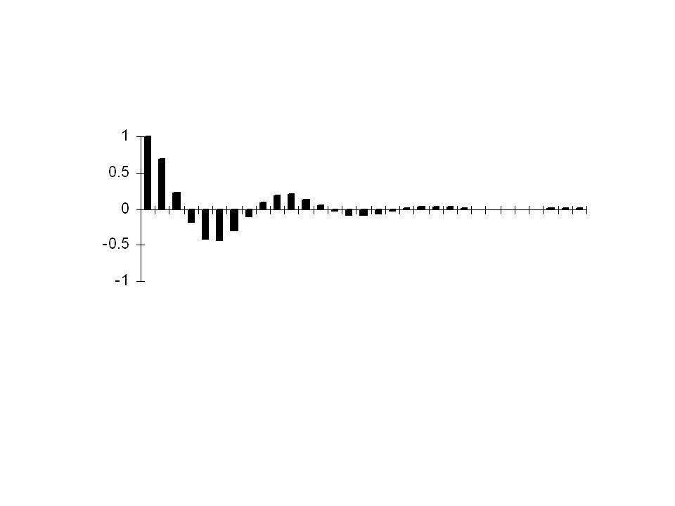
23. The autocorrelation function: This statistic measures the correlation between residuals the occur a distance k apart in time. One would expect that residuals that are close in time are more correlated than residuals that are separated by a greater distance in time. If the residuals are independent than r k should be close to zero for all values of k A plot of r k versus k can be very revealing with respect to the independence of the residuals. Some typical patterns of the autocorrelation function are given below: The autocorrelation function at lag k is defined by :

24. This statistic measures the correlation between residuals the occur a distance k apart in time. One would expect that residuals that are close in time are more correlated than residuals that are separated by a greater distance in time. If the residuals are independent than r k should be close to zero for all values of k A plot of r k versus k can be very revealing with respect to the independence of the residuals.

25. Some typical patterns of the autocorrelation function are given below: Auto correlation pattern for independent residuals

26. Various Autocorrelation patterns for serially correlated residuals

28. The runs test: This test uses the fact that the residuals will oscillate about zero at a “normal” rate if the random departures are independent. If the residuals oscillate slowly about zero, this is an indication that there is a positive autocorrelation amongst the residuals. If the residuals oscillate at a frequent rate about zero, this is an indication that there is a negative autocorrelation amongst the residuals.

29. In the “runs test”, one observes the time sequence of the “sign” of the residuals: + + + - - + + - - - + + + and counts the number of runs (i.e. the number of periods that the residuals keep the same sign). This should be low if the residuals are positively correlated and high if negatively correlated.

30. Plot Against fitted values and the Predictor Variables X ij If we "step back" from this diagram and the residuals behave in a manner consistent with the assumptions of the model we obtain the impression of a horizontal "band " of residuals which can be represented by the diagram below.

31. Individual observations lying considerably outside of this band indicate that the observation may be and outlier. An outlier is an observation that is not following the normal pattern of the other observations. Such an observation can have a considerable effect on the estimation of the parameters of a model. Sometimes the outlier has occurred because of a typographical error. If this is the case and it is detected than a correction can be made. If the outlier occurs for other (and more natural) reasons it may be appropriate to construct a model that incorporates the occurrence of outliers.

32. If our "step back" view of the residuals resembled any of those shown below we should conclude that assumptions about the model are incorrect. Each pattern may indicate that a different assumption may have to be made to explain the “abnormal” residual pattern. b) a)

33. Pattern a) indicates that the variance the random departures is not constant (homogeneous) but increases as the value along the horizontal axis increases (time, or one of the independent variables). This indicates that a weighted least squares analysis should be used. The second pattern, b) indicates that the mean value of the residuals is not zero. Linear and quadratic terms have been omitted that should have been included in the model. This is usually because the model (linear or non linear) has not been correctly specified.

34. Example – Analysis of Residuals Motor Vehicle Data Dependent = mpg Independent = Engine size, horsepower and weight

35. When a linear model was fit and residuals examined graphically the following plot resulted:

36. The pattern that we are looking for is:

37. The pattern that was found is: This indicates a nonlinear relationship: This can be handle by adding polynomial terms (quadratic, cubic, quartic etc.) of the independent variables or transforming the dependent variable

38. Performing the log transformation on the dependent variable (mpg) results in the following residual plot There still remains some non linearity

39. The log transformation

40. The Box-Cox transformations = 2 = 0 = -1 = 1 = -1

41. The log ( = 0) transformation was not totally successful - try moving further down the staircase of the family of transformations ( = -0.5)

42. try moving a bit further down the staircase of the family of transformations ( = -1.0)

43. The results after deleting the outlier are given below:

44. This corresponds to the model or and

45. Checking normality with a P-P plot

46. Example Non-Linear Regression

47. In this example we are measuring the amount of a compound in the soil: 1.7 days after application 2.14 days after application 3.21 days after application 4.28 days after application 5.42 days after application 6.56 days after application 7.70 days after application 8.84 days after application

48. This is carried out at two test plot locations 1.Craik 2.Tilson 6 measurements per location are made each time

49. The data

50. Graph

51. The Model: Exponential decay with nonzero asymptote c a

52. Some starting values of the parameters found by trial and error by Excel

53. Non Linear least squares iteration by SPSS (Craik)

54. ANOVA Table (Craik) Parameter Estimates (Craik)

55. Testing Hypothesis: similar to linear regression Caution: This statistic has only an approximate F – distribution when the sample size is large

56. Example: Suppose we want to test H 0 : c = 0 against H A : c ≠ 0 Complete model Reduced model

57. ANOVA Table (Complete model) ANOVA Table (Reduced model)

58. The Test

59. Use of Dummy Variables Non Linear Regression

60. The Model: or where

61. The data file

62. Non Linear least squares iteration by SPSS

63. ANOVA Table Parameter Estimates

64. Testing Hypothesis: Suppose we want to test H 0 :  a = a 1 – a 2 = 0 and  k = k 1 – k 2 = 0

65. The Reduced Model: or

66. ANOVA Table Parameter Estimates

67. The F Test Thus we accept the null Hypothesis that the reduced model is correct

69. Factorial Experiments Analysis of Variance Experimental Design

70. Dependent variable Y k Categorical independent variables A, B, C, … (the Factors) Let –a = the number of categories of A –b = the number of categories of B –c = the number of categories of C –etc.

71. The Completely Randomized Design We form the set of all treatment combinations – the set of all combinations of the k factors Total number of treatment combinations –t = abc…. In the completely randomized design n experimental units (test animals, test plots, etc. are randomly assigned to each treatment combination. –Total number of experimental units N = nt=nabc..

72. The treatment combinations can thought to be arranged in a k-dimensional rectangular block A 1 2 a B 12b

73. A B C

74. The Completely Randomized Design is called balanced If the number of observations per treatment combination is unequal the design is called unbalanced. (resulting mathematically more complex analysis and computations) If for some of the treatment combinations there are no observations the design is called incomplete. (some of the parameters - main effects and interactions - cannot be estimated.)

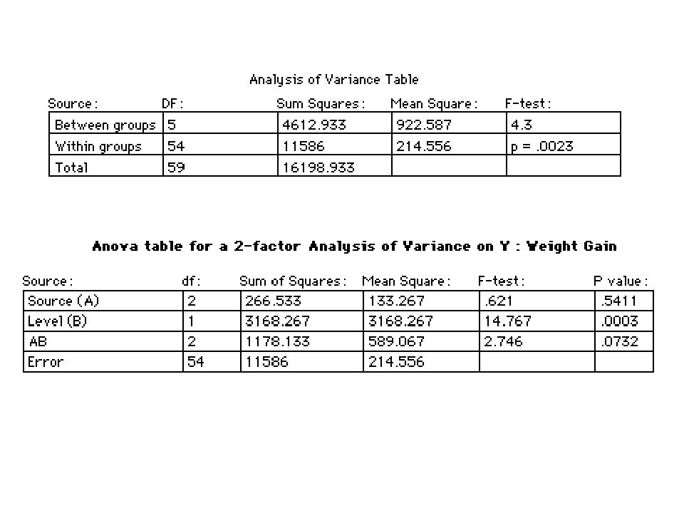
75. Example In this example we are examining the effect of We have n = 10 test animals randomly assigned to k = 6 diets tThe level of protein A (High or Low) and tThe source of protein B (Beef, Cereal, or Pork) on weight gains (grams) in rats.

76. The k = 6 diets are the 6 = 3×2 Level-Source combinations 1.High - Beef 2.High - Cereal 3.High - Pork 4.Low - Beef 5.Low - Cereal 6.Low - Pork

77. Table Gains in weight (grams) for rats under six diets differing in level of protein (High or Low) and s ource of protein (Beef, Cereal, or Pork) Level of ProteinHigh ProteinLow protein Source of ProteinBeefCerealPorkBeefCerealPork Diet123456 7398949010749 1027479769582 1185696909773 10411198648086 8195102869881 10788102517497 100821087274106 877791906770 11786120958961 11192105785882 Mean100.085.999.579.283.978.7 Std. Dev.15.1415.0210.9213.8915.7116.55

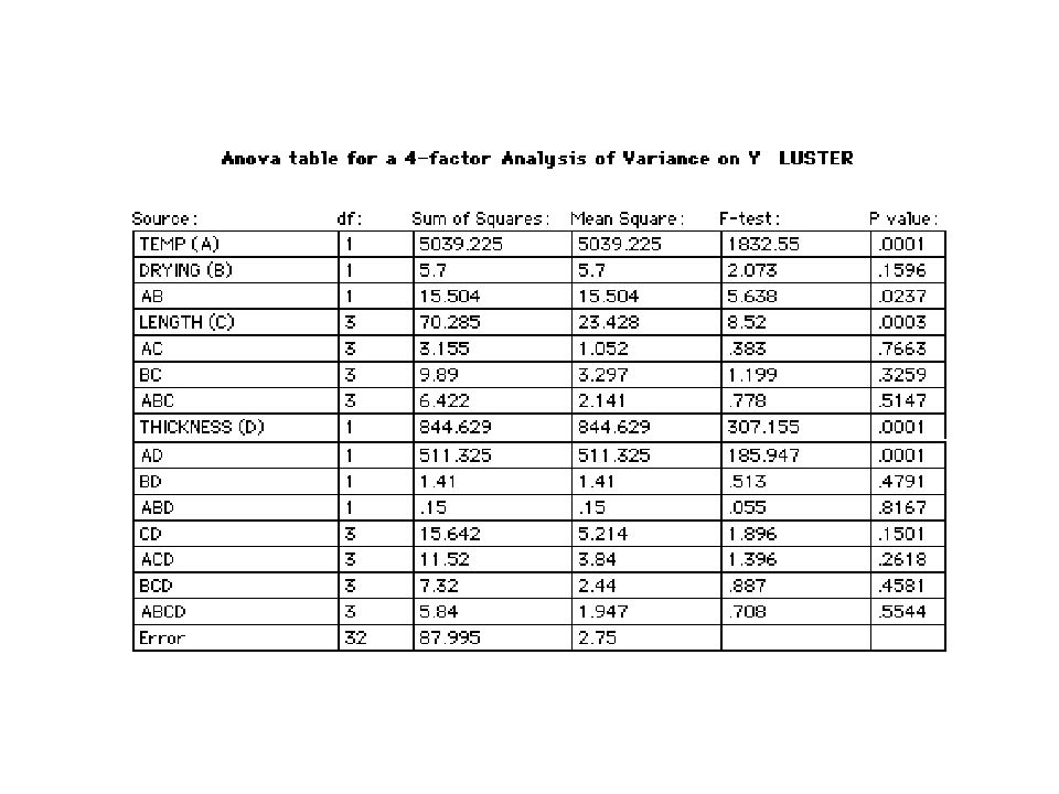
78. Example – Four factor experiment Four factors are studied for their effect on Y (luster of paint film). The four factors are: Two observations of film luster (Y) are taken for each treatment combination 1) Film Thickness - (1 or 2 mils) 2)Drying conditions (Regular or Special) 3)Length of wash (10,30,40 or 60 Minutes), and 4)Temperature of wash (92 ˚C or 100 ˚C)

79. The data is tabulated below: Regular DrySpecial Dry Minutes92  C100  C92  C100  C 1-mil Thickness 203.43.419.614.52.13.817.213.4 304.14.117.517.04.04.613.514.3 404.94.217.615.25.13.316.017.8 605.04.920.917.18.34.317.513.9 2-mil Thickness 205.53.726.629.54.54.525.622.5 305.76.131.630.25.95.929.229.8 405.55.630.530.25.55.832.627.4 607.26.031.429.68.09.933.529.5

80. Notation Let the single observations be denoted by a single letter and a number of subscripts y ijk…..l The number of subscripts is equal to: (the number of factors) + 1 1 st subscript = level of first factor 2 nd subscript = level of 2 nd factor … Last subsrcript denotes different observations on the same treatment combination

81. Notation for Means When averaging over one or several subscripts we put a “bar” above the letter and replace the subscripts by  Example: y 241   

82. Profile of a Factor Plot of observations means vs. levels of the factor. The levels of the other factors may be held constant or we may average over the other levels

83. Level of ProteinBeefCerealPorkOverall Low79.2083.9078.7080.60 Source of Protein High100.0085.9099.5095.13 Overall89.6084.9089.1087.87 Summary Table

84. Profiles of Weight Gain for Source and Level of Protein

86. Effects in a factorial Experiment

87. Mean 87.867

88. Main Effects for Factor A (Source of Protein) BeefCerealPork 1.733-2.9671.233

89. Main Effects for Factor B (Level of Protein) HighLow 7.267-7.267

90. AB Interaction Effects Source of Protein BeefCerealPork LevelHigh3.133-6.2673.133 of Protein Low-3.1336.267-3.133

92. Example 2 Paint Luster Experiment

94. Table: Means and Cell Frequencies

95. Means and Frequencies for the AB Interaction (Temp - Drying)

96. Profiles showing Temp-Dry Interaction

97. Means and Frequencies for the AD Interaction (Temp- Thickness)

98. Profiles showing Temp-Thickness Interaction

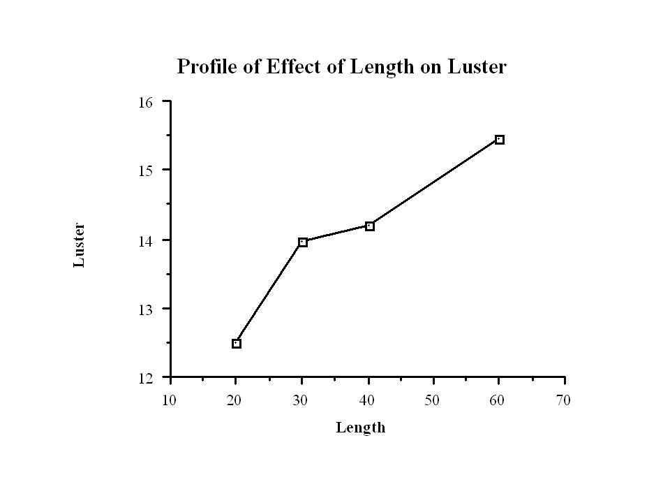
99. The Main Effect of C (Length)

101. Additive Factors A B

102. Interacting Factors A B

103. Models for factorial Experiments Single Factor: y ij =  +  i +  ij i = 1,2,...,a; j = 1,2,...,n Two Factor: y ijk =  +  i +  j +  ij +  ijk i = 1,2,...,a ; j = 1,2,...,b ; k = 1,2,...,n

104. Three Factor: y ijkl =  +  i +  j +  ij +  k + (  ik + (  jk +  ijk +  ijkl =  +  i +  j +  k +  ij + (  ik + (  jk +  ijk +  ijkl i = 1,2,...,a ; j = 1,2,...,b ; k = 1,2,...,c; l = 1,2,...,n

105. Four Factor: y ijklm =  +  i +  j +  ij +  k + (  ik + (  jk +  ijk +  l + (  il + (  jl +  ijl + (  kl + (  ikl + (  jkl +  ijkl +  ijklm =  +  i +  j +  k +  l +  ij + (  ik + (  jk + (  il + (  jl + (  kl +  ijk +  ijl + (  ikl + (  jkl +  ijkl +  ijklm i = 1,2,...,a ; j = 1,2,...,b ; k = 1,2,...,c; l = 1,2,...,d; m = 1,2,...,n where0 =   i =   j =   ij =   k =  (  ik =  (  jk =   ijk =   l =  (  il =  (  jl =   ijl =  (  kl =  (  ikl =  (  jkl =   ijkl and  denotes the summation over any of the subscripts.

106. Estimation of Main Effects and Interactions Estimator of Main effect of a Factor Estimator of k-factor interaction effect at a combination of levels of the k factors = Mean at the combination of levels of the k factors - sum of all means at k-1 combinations of levels of the k factors +sum of all means at k-2 combinations of levels of the k factors - etc. =Mean at level i of the factor - Overall Mean

107. Example: The main effect of factor B at level j in a four factor (A,B,C and D) experiment is estimated by: The two-factor interaction effect between factors B and C when B is at level j and C is at level k is estimated by:

108. The three-factor interaction effect between factors B, C and D when B is at level j, C is at level k and D is at level l is estimated by: Finally the four-factor interaction effect between factors A,B, C and when A is at level i, B is at level j, C is at level k and D is at level l is estimated by:

109. Definition: A factor is said to not affect the response if the profile of the factor is horizontal for all combinations of levels of the other factors: No change in the response when you change the levels of the factor (true for all combinations of levels of the other factors) Otherwise the factor is said to affect the response:

110. Definition: Two (or more) factors are said to interact if changes in the response when you change the level of one factor depend on the level(s) of the other factor(s). Profiles of the factor for different levels of the other factor(s) are not parallel Otherwise the factors are said to be additive. Profiles of the factor for different levels of the other factor(s) are parallel.

111. If two (or more) factors interact each factor effects the response. If two (or more) factors are additive it still remains to be determined if the factors affect the response In factorial experiments we are interested in determining –which factors effect the response and – which groups of factors interact.

112. The testing in factorial experiments 1.Test first the higher order interactions. 2.If an interaction is present there is no need to test lower order interactions or main effects involving those factors. All factors in the interaction affect the response and they interact 3.The testing continues with for lower order interactions and main effects for factors which have not yet been determined to affect the response.

113. Models for factorial Experiments Single Factor: y ij =  +  i +  ij i = 1,2,...,a; j = 1,2,...,n Two Factor: y ijk =  +  i +  j +  ij +  ijk i = 1,2,...,a ; j = 1,2,...,b ; k = 1,2,...,n

114. Three Factor: y ijkl =  +  i +  j +  ij +  k + (  ik + (  jk +  ijk +  ijkl =  +  i +  j +  k +  ij + (  ik + (  jk +  ijk +  ijkl i = 1,2,...,a ; j = 1,2,...,b ; k = 1,2,...,c; l = 1,2,...,n

115. Four Factor: y ijklm =  +  i +  j +  ij +  k + (  ik + (  jk +  ijk +  l + (  il + (  jl +  ijl + (  kl + (  ikl + (  jkl +  ijkl +  ijklm =  +  i +  j +  k +  l +  ij + (  ik + (  jk + (  il + (  jl + (  kl +  ijk +  ijl + (  ikl + (  jkl +  ijkl +  ijklm i = 1,2,...,a ; j = 1,2,...,b ; k = 1,2,...,c; l = 1,2,...,d; m = 1,2,...,n where0 =   i =   j =   ij =   k =  (  ik =  (  jk =   ijk =   l =  (  il =  (  jl =   ijl =  (  kl =  (  ikl =  (  jkl =   ijkl and  denotes the summation over any of the subscripts.

116. Estimation of Main Effects and Interactions Estimator of Main effect of a Factor Estimator of k-factor interaction effect at a combination of levels of the k factors = Mean at the combination of levels of the k factors - sum of all means at k-1 combinations of levels of the k factors +sum of all means at k-2 combinations of levels of the k factors - etc. =Mean at level i of the factor - Overall Mean

117. Example: The main effect of factor B at level j in a four factor (A,B,C and D) experiment is estimated by: The two-factor interaction effect between factors B and C when B is at level j and C is at level k is estimated by:

118. The three-factor interaction effect between factors B, C and D when B is at level j, C is at level k and D is at level l is estimated by: Finally the four-factor interaction effect between factors A,B, C and when A is at level i, B is at level j, C is at level k and D is at level l is estimated by:

119. Anova Table entries Sum of squares interaction (or main) effects being tested  (product of sample size and levels of factors not included in the interaction) Degrees of freedom = df = product of (number of levels - 1) of factors included in the interaction.

120. Mean 87.867

121. Main Effects for Factor A (Source of Protein) BeefCerealPork 1.733-2.9671.233

122. Main Effects for Factor B (Level of Protein) HighLow 7.267-7.267

123. AB Interaction Effects Source of Protein BeefCerealPork LevelHigh3.133-6.2673.133 of Protein Low-3.1336.267-3.133

126. Table: Means and Cell Frequencies

127. Means and Frequencies for the AB Interaction (Temp - Drying)

128. Profiles showing Temp-Dry Interaction

129. Means and Frequencies for the AD Interaction (Temp- Thickness)

130. Profiles showing Temp-Thickness Interaction

131. The Main Effect of C (Length)