1. Experimental Statistics - week 9
Chapter 18:
Repeated Measures

2. Repeated Measures with a Single Factor
Time
Subject
Reading for
ith time period
jth subject

3. Single Factor Repeated Measures Designs
single factor repeated measures model is similar to the randomized complete block model
- i.e. 2 factors (subject and time) with one observation cell
- since there is only one observation per cell, we cannot estimate an interaction term
typically:
- subject is a random effect
- time is a fixed effect
time
subject

4. Repeated Measure Design with Single Factor
ANOVA Table for
Repeated Measure Design with Single Factor
Source SS df MS EMS F
Between subjects SSP n MSP MSP/MSE
  Time SSA a MSA MSA/MSE
Error SSE (n - 1)(a- 1) MSE
Total TSS an - 1

5. Data – 5 subjects take tablet
-- blood samples taken .5, 1, 2, 3, and 4 hours after ingestion
Goal: understand rate at which medicine enters blood
Time
Subject

6. Dependent Variable: conc
Sum of
Source DF Squares Mean Square F Value Pr > F
Model <.0001
Error
Corrected Total
R-Square Coeff Var Root MSE conc Mean
Source DF Type III SS Mean Square F Value Pr > F
subject
time <.000

7. The GLM Procedure
t Tests (LSD) for conc
NOTE: This test controls the Type I comparisonwise error rate, not the experimentwise error rate.
Alpha
Error Degrees of Freedom
Error Mean Square
Critical Value of t
Least Significant Difference
Means with the same letter are not significantly different.
t Group Mean N time A B B B C D

9. Results:

10. Residual Diagnostics – 1-factor Repeated Measures Data

11. Note:
An additional assumption (related to the equal variance assumption) is that of sphericity
-- the assumption that pairwise differences between times all have the same population variances
-- compound symmetry is a related (more stringent) requirement
-- discussed briefly in text
-- beyond scope of this course

12. Two-Factor Repeated Measure Data (p.1033)
Data – 10 subjects (5 take tablet, 5 take capsule)
-- blood samples .5, 1, 2, 3, and 4 hours after ingestion
Goal: compare blood concentration patterns of the two methods of administration
Tablet
Capsule
Time
Subject
Time
Subject

13. 2-Factor with Repeated Measure -- Model
type
subject within type
type by time interaction
time
NOTES: type and time are both fixed effects in the current example
- we say “subject is nested within type”
- Expected Mean Squares given on page 1032

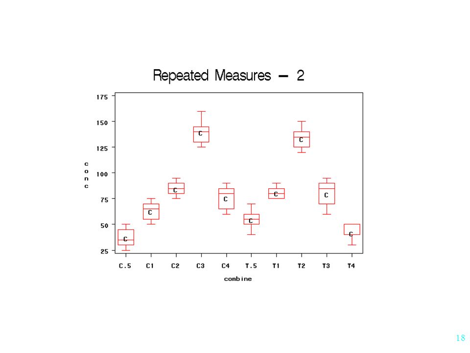
14. PROC GLM;
CLASS type subject time;
MODEL conc=type subject(type) time type*time;
TITLE 'Repeated Measures – 2 factors';
OUTPUT out=new r=resid;
MEANS type time/LSD;
RANDOM subject(type)/test;

15. 2-Factor Repeated Measures – ANOVA Output
The GLM Procedure
Dependent Variable: conc
Sum of
Source DF Squares Mean Square F Value Pr > F
Model <.0001
Error
Corrected Total
R-Square Coeff Var Root MSE conc Mean
Source DF Type III SS Mean Square F Value Pr > F
type
subject(type) <.0001
time <.0001
type*time <.0001

16. 2-factor Repeated Measures
Source Type III Expected Mean Square
type Var(Error) + 5 Var(subject(type)) + Q(type,type*time)
subject(type) Var(Error) + 5 Var(subject(type))
time Var(Error) + Q(time,type*time)
type*time Var(Error) + Q(type*time)
The GLM Procedure
Tests of Hypotheses for Mixed Model Analysis of Variance
Dependent Variable: conc
Source DF Type III SS Mean Square F Value Pr > F
* type
Error
Error: MS(subject(type))
* This test assumes one or more other fixed effects are zero.
Source DF Type III SS Mean Square F Value Pr > F
subject(type) <.0001
* time <.0001
type*time <.0001
Error: MS(Error)

17. NOTE: Since time x type interaction is significant, and since these are fixed effects we DO NOT test main effects
– we compare cell means (using MSE)
Cell Means C T

19. Note on Multiple Comparisons:
If there had NOT been a significant interaction, then the LSD to compare cell means:
(a) for time – use MSE
(SAS will give these results)
(b) for type – use MS(subject(type))
(SAS will NOT give these results)

20. SAS LSD Output for Comparing Times
Alpha
Error Degrees of Freedom
Error Mean Square
Critical Value of t
Least Significant Difference
Means with the same letter are not significantly different.
t Grouping Mean N time A A A B C D

21. Diagnostic Plots for 2-Factor Repeated Measures Data

22. Write-up related to the SAS output.

23. Note, that even though we get a significant variance component due to subject(within group) I did not estimate the variance component itself. (I did not give this particular variance component estimation formula.)

24. Dealing with Normality/Equal Variance Issues
Normalizing Transformations:
- log
- square root
- Box-Cox transformations
Note: the normalizing transformations sometimes also produce variance stabilization

25. Nonparametric “ANOVA”
Man-Whitney U – for comparing 2 independent samples
Kruskal-Wallis Test – for comparing >2 independent samples
Friedman’s Test – nonparametric alternative to randomized complete block/ factor repeated measures design

26. Section 2 Regression Analysis

27. Scatter Diagram (Scatterplot)
Histogram
displays distribution of 1 variable
Scatter Diagram (Scatterplot)
displays joint distribution of 2 variables
plots data as “points” in the “x-y plane.”

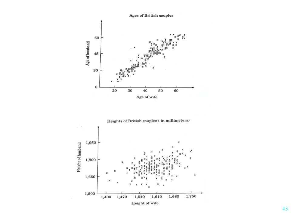
30. Association Between Two Variables
indicates that knowing one helps in predicting the other
Linear Association
our interest in this course
points “swarm” about a line
Correlation Analysis
measures the strength of linear association

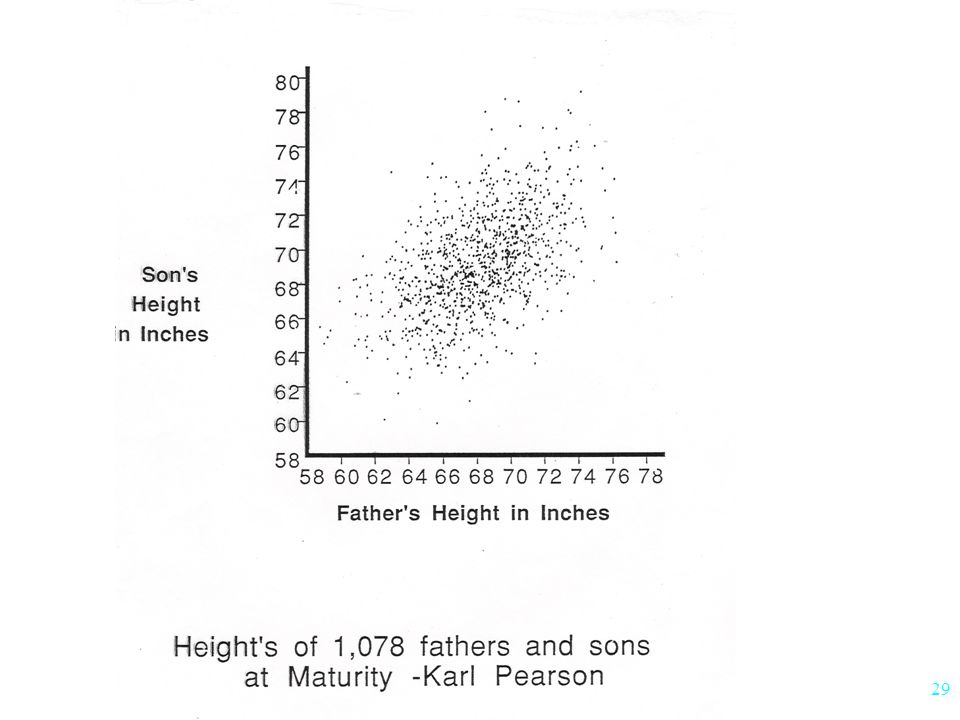
31. Hypothetical Father-Son Data
Son’s
Height
in Inches
Father’s Height in Inches

32. (association)

33. Regression Analysis Dependent Variable (Y) Independent Variable (X)
We want to predict the dependent variable
- response variable
using the independent variable
- explanatory variable
- predictor variable
Dependent
Variable
(Y)
Independent Variable (X)
More than one independent variable – Multiple Regression

34. 11.7 Correlation Analysis

35. Correlation Coefficient - measures linear association
perfect no perfect
negative linear positive
relationship relationship relationship
Denoted r or ryx

36. Positive Correlation - - high values of one variable are associated with high values of the other3 2 1
Examples:
- father’s height, son’s height
- daily grade, final grade
r = 0.93 for plot on the left

37. EXAMS I and II

38. Negative Correlation - - high with low, low with high
Examples:
- car age, selling price
- days absent, final grade
r = for plot shown here 4 3 2 1

40. Zero Correlation - - no linear relationship5 4 3 2 1
Examples:
- height, IQ score
r = 0.0 for plot here

42. -.75, 0, .5, .99

44. Calculating the Correlation Coefficient

45. Notation:
So --

46. Find r The data below are the study times and the test scores
on an exam given over the material covered during the two weeks.
Study Time Exam
(hours) Score
(X) (Y)
Find r

47. DATA one;
INPUT time score;
DATALINES;
10 92
15 81
12 84
20 74
8 85
16 80
14 84
22 80 ;
PROC CORR;
Var score time;
TITLE ‘Study Time by Score';
RUN;
PROC PLOT;
PLOT time*score;
PROC GPLOT;

48. The CORR Procedure
2 Variables: score time
Simple Statistics
Variable N Mean Std Dev Sum Minimum Maximum
score
time
Pearson Correlation Coefficients, N = 8
Prob > |r| under H0: Rho=0
score time
score
0.0239
time
Study Time by Score

49. PROC PLOT Plot of score*time. Legend: A = 1 obs, B = 2 obs, etc.‚
92 ˆ A
91 ˆ
90 ˆ
89 ˆ
88 ˆ
87 ˆ
86 ˆ
85 ˆ A
84 ˆ A A
83 ˆ
82 ˆ
81 ˆ A
80 ˆ A A
79 ˆ
78 ˆ
77 ˆ
76 ˆ
75 ˆ
74 ˆ A
Šƒƒˆƒƒƒƒƒˆƒƒƒƒƒˆƒƒƒƒƒˆƒƒƒƒƒˆƒƒƒƒƒˆƒƒƒƒƒˆƒƒƒƒƒˆƒƒƒƒƒˆƒƒƒƒƒˆƒƒƒƒƒˆƒƒƒƒƒˆƒƒƒƒƒˆƒƒƒƒƒˆƒƒƒƒƒˆƒƒ
time

50. PROC GPLOT