Download presentation
Presentation is loading. Please wait.

1
Environmental and Exploration Geophysics II tom.h.wilson wilson@geo.wvu.edu Department of Geology and Geography West Virginia University Morgantown, WV Common MidPoint (CMP) Records and Stacking
 Records and Stacking")
2
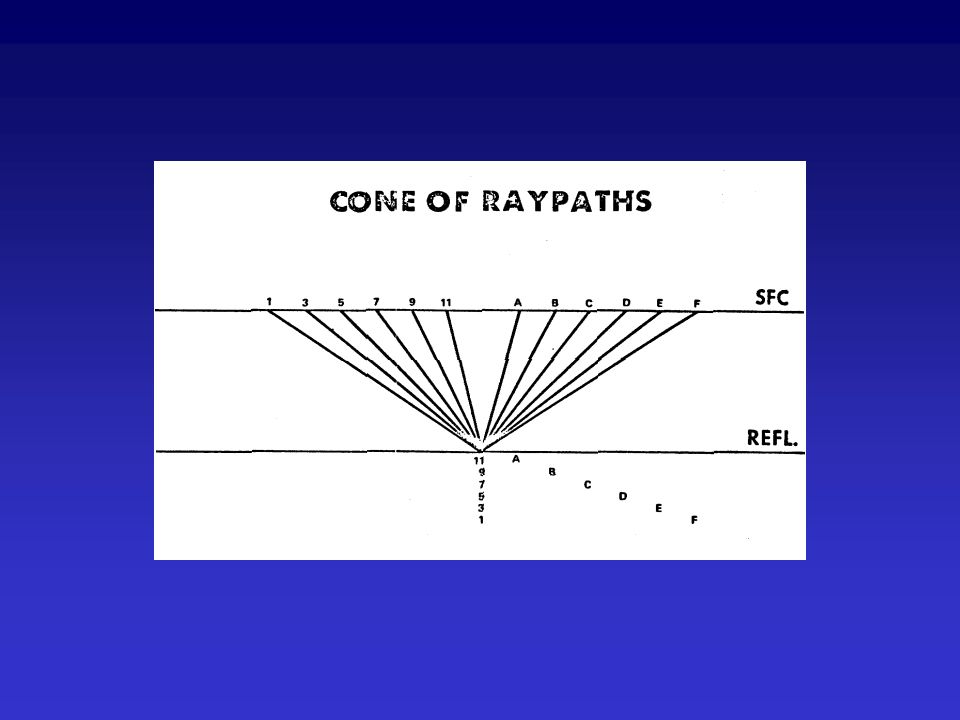
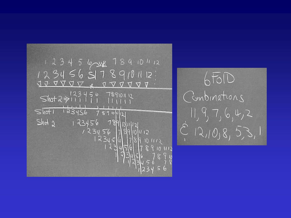
Stacking Chart - 3 fold Fold refers to the redundancy in reflection point coverage

3
Off-end 12 geophone source receiver layout

4
Drag receiver string to the right ->

8
Moveout in the common midpoint gather is hyperbolic

9
regardless of whether the layer is flat lying or dipping.

10
Along crooked survey lines, the common midpoint gather includes all records whose midpoints fall within a certain radius of some point Crooked Line Effects

12
NMO corrections to the arrivals in a common- midpoint gather yield the same coincidence of sources and receivers, but in this case all sources and receivers relocate to the same midpoint.

14
Let’s assume that the traces shown at right are nmo corrected traces in a common midpoint gather. They are all identical. However, the real world doesn’t work this way. We always have noise in our data. Source Receiver Offset ->

15
Here’s the same data set with a lot of noise thrown in. Note so easy to see the signal in this case - is it? Pure signalNoisy signal

16
Greenbrier Huron Onondaga

17
If we sum all the noisy traces together - sample by sample - we get the trace plotted in the gap at right. This summation of all 16 traces is referred to as a stack trace. Note that the stack trace compares quite well with the pure signal. Stack Trace

18
+1 Noise comes in several forms - both coherent and random. Coherent noise may come in the form of some unwanted signal such as ground roll. A variety of processing and acquisition techniques have been developed to reduce the influence of coherent noise. The basic nature of random noise can be described in the context of a random walk - Random noise can come in the form of wind, rain, mining activities, local traffic, microseismicity... See the Feynman Lectures on Physics, Volume 1.

19
The random walk attempts to follow the progress one achieves by taking steps in the positive or negative direction purely at random - to be determined, for example, by a coin toss. +1

20
Does the walker get anywhere? Our intuition tells us that the walker should get nowhere and will simply wonder about their point of origin. However, lets take a look at the problem form a more quantitative view. It is easy to keep track of the average distance the walker departs from their starting position by following the behavior of the average of the square of the departure. We write the average of the square of the distance from the starting point after N steps as The average is taken over several repeated trials.

21
After 1 step will always equal 1 ( the average of +1 2 or -1 2 is always 1. After two steps - which is 0 or 4 so that the average is 2. After N steps

22
Averaged over several attempts to get home the wayward wonderer gets on average to a distance squared from the starting point. Since=1, it follows that and therefore that

23
The results of three sets of random coin toss experiments

24
The implications of this simple problem to our study of seismic methods relates to the result obtained through stacking of the traces in the common midpoint gather. The random noise present in each trace of the gather (plotted at left) has been partly but not entirely eliminated in the stack trace. Just as in the case of the random walk, the noise appearing in repeated recordings at the same travel time, although random, does not completely cancel out
 has been partly but not entirely eliminated in the stack trace. Just as in the case of the random walk, the noise appearing in repeated recordings at the same travel time, although random, does not completely cancel out.")
25
The relative amplitude of the noise - analogous to the distance traveled by our random walker- does not drop to zero but decreases in amplitude relative to the signal. If N traces are summed together, the amplitude of the resultant signal will be N times its original value since the signal always arrives at the same time and sums together constructively. The amplitude of noise on the other hand because it is a random process increases as Hence, the ratio of signal to noise isor just where N is the number of traces summed together or the number of traces in the CMP gather.

26
In the example at left, the common midpoint gather consists of 16 independent recordings of the same reflection point. The signal-to-noise ratio in the stack trace has increased by a factor of 16 or 4. The number of traces that are summed together in the stack trace is referred to as its fold.

27
If you had a 20 fold dataset and wished to improve its signal-to-noise ratio by a factor of 2, what fold data would be required? Square root of 20 = 4.472 Square root of N(?) = 8.94 What’s N To double the signal to noise ratio we must quadruple the fold
 = 8.94 What’s N To double the signal to noise ratio we must quadruple the fold.")
28
The reliability of the output stack trace is critically dependant on the accuracy of the correction velocity.

29
Accurate correction ensures that the same part of adjacent waveforms are summed together in phase. Average Amplitude

30
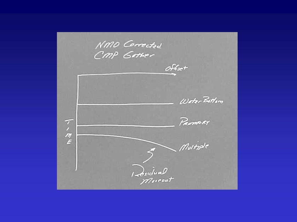
If the correction velocity is in error then the reflection response will be “smeared out” in the stack trace through destructive interference between traces in the sum.

31
The two-term approximation to the multilayer reflection response is hyperbolic. The velocity in this expression is a root-mean-square velocity. Are they also hyperbolic?

32
The sum of squared velocity is weighted by the two- way interval transit times t i through each layer. ignore

33
The approximation is hyperbolic, whereas the actual is not. The disagreement becomes significant at longer offsets, where the actual reflection arrivals often come in earlier that those predicted by the hyperbolic approximation.

34
The reason for this becomes obvious when you think of the earth as consisting of layers of increasing velocity. At larger and larger incidence angle you are likely to come in at near critical angles and then will travel significant distances at higher than average (or RMS) velocity. Greenbrier Limestone Big Injun
 velocity. Greenbrier Limestone Big Injun.")
35
We make a point of noting and comparing the V RMS V AV and V NMO because the V NMO is often taken to be the V RMS. However, each of these 3 velocities has different geometrical significance.

36
The V NMO is derived form the slope of the regression line fit to the actual arrivals. In actuality the moveout velocity varies with offset. The RMS velocity corresponds to the square root of the reciprocal of the slope of the t 2 -x 2 curve for relatively short offsets.

37
The general relationship between the average, RMS and NMO velocities is shown at right.

38
Geometrically the average velocity characterizes travel along the normal incidence path. The RMS velocity describes travel times through a single layer having the RMS velocity. It ignores refraction across individual layers.

41
DEPTHDEPTH

45
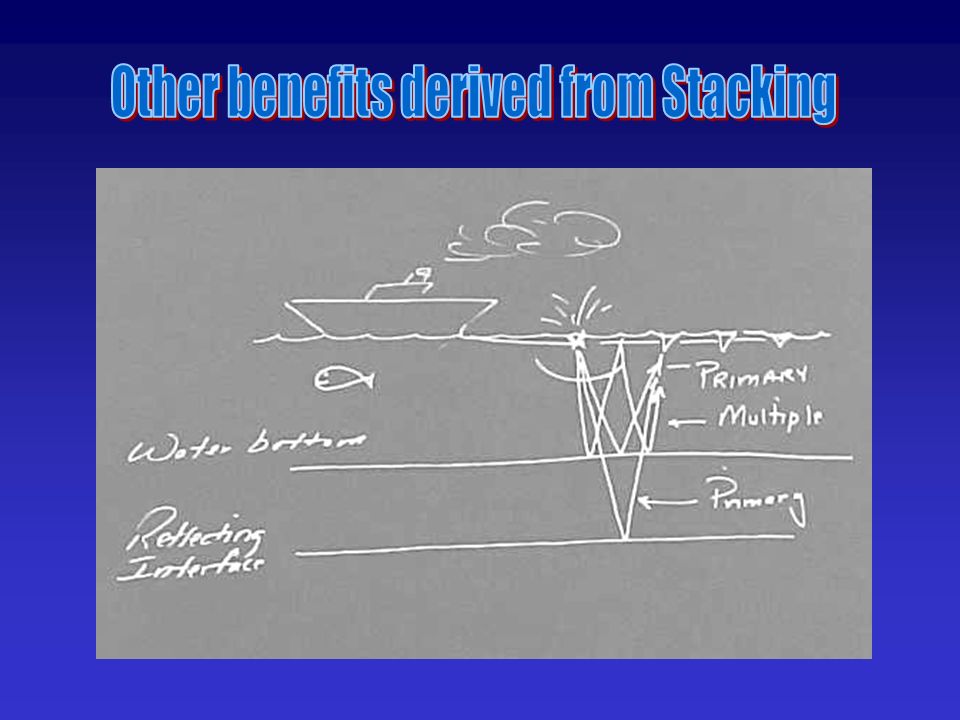
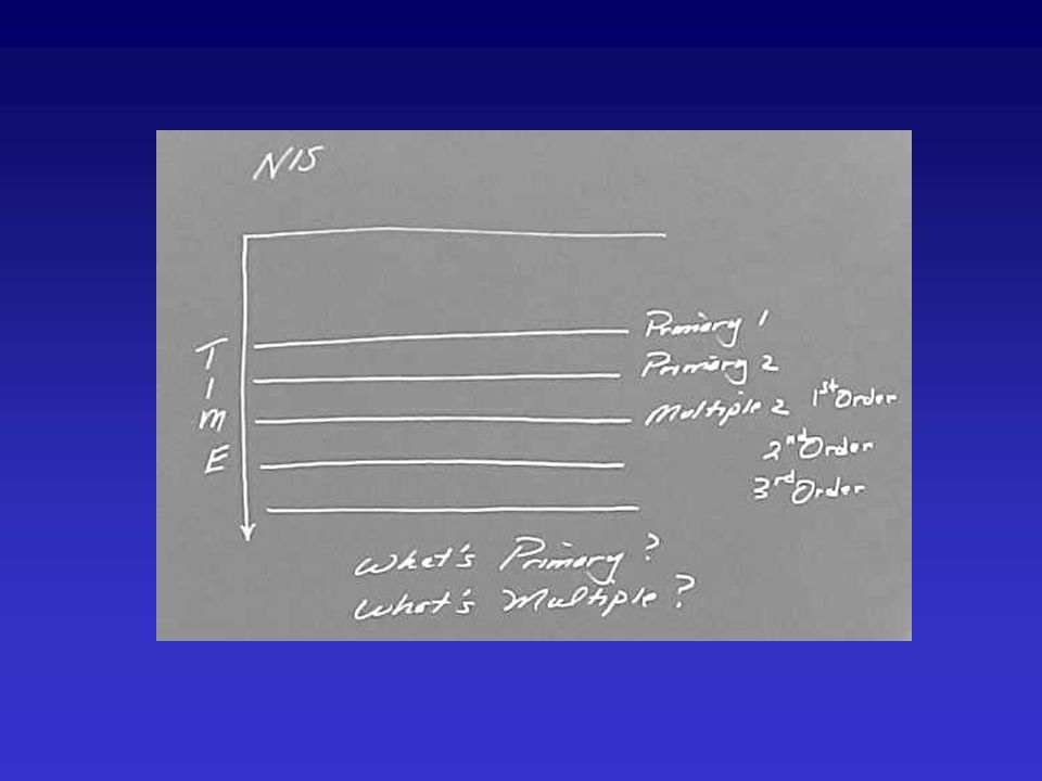
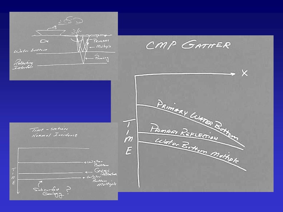
Multiple attenuation Multiple Primary Reflections

46
Buried graben or multiple

47
Multiples are considered “coherent” noise or unwanted signal

48
Interbed multiple or Stacked pays

50
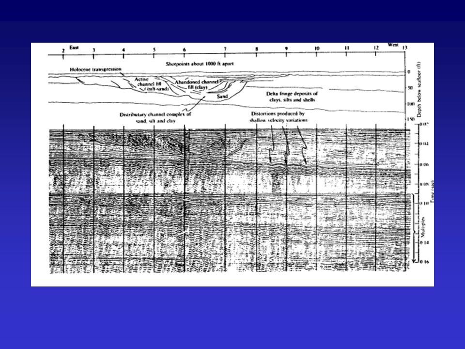
Waterbottom and sub-bottom multiples

51
Other forms of coherent “noise” will also be attenuated by the stacking process. The displays at right are passive recordings (no source) of the background noise. The hyperbolae you see are associated with the movement of an auger along a panel face of a longwall mine.
 of the background noise. The hyperbolae you see are associated with the movement of an auger along a panel face of a longwall mine..")
52
Multiples Refractions Air waves Ground Roll Streamer cable motion Scattered waves from off line

53
Today Due today Today

Similar presentations