2. MULTIDIMENSIONAL HEAT TRANSFER  This equation governs the Cartesian, temperature distribution for a three-dimensional unsteady, heat transfer problem involving heat generation.  For steady state  /  t = 0  No generation  To solve for the full equation, it requires a total of six boundary conditions: two for each direction. Only one initial condition is needed to account for the transient behavior.

3. Two-Dimensional, Steady State Case There are three approaches to solve this equation:  Numerical Method: Finite difference or finite element schemes, usually will be solved using computers.  Graphical Method: Limited use. However, the conduction shape factor concept derived under this concept can be useful for specific configurations. (see Table 4.1 for selected configurations)  Analytical Method: The mathematical equation can be solved using techniques like the method of separation of variables. (refer to handout)

4. Conduction Shape Factor  This approach applied to 2-D conduction involving two isothermal surfaces, with all other surfaces being adiabatic. The heat transfer from one surface (at a temperature T 1 ) to the other surface (at T 2 ) can be expressed as: q=Sk(T 1 -T 2 ) where k is the thermal conductivity of the solid and S is the conduction shape factor.  The shape factor can be related to the thermal resistance: q=Sk(T 1 - T 2 )=(T 1 -T 2 )/(1/kS)= (T 1 -T 2 )/R t where R t = 1/(kS)  1-D heat transfer can use shape factor also. Ex: Heat transfer inside a plane wall of thickness L is q=kA(  T/L), S=A/L  Common shape factors for selected configurations can be found in most textbooks, as also illustrated in Table 4.1.

7. Example Example: A 10 cm OD uninsulated pipe carries steam from the power plant across campus. Find the heat loss if the pipe is buried 1 m in the ground is the ground surface temperature is 50 ºC. Assume a thermal conductivity of the sandy soil as k = 0.52 w/m K. z=1 m T2T2 T1T1

8. The shape factor for long cylinders is found in Table 4.1 as Case 2, with L >> D: S = 2  L/ln(4  z/D) Where z = depth at which pipe is buried. S = 2  1  m/ln(40) = 1.7 m Then q' = (1.7  m)(0.52 W/m  K)(100 o C - 50 o C) q' = 44.2 W

9. Numerical Methods  Due to the increasing complexities encountered in the development of modern technology, analytical solutions usually are not available. For these problems, numerical solutions obtained using high-speed computer are very useful, especially when the geometry of the object of interest is irregular, or the boundary conditions are nonlinear. In numerical analysis, three different approaches are commonly used: the finite difference, the finite volume and the finite element methods. In heat transfer problems, the finite difference and finite volume methods are used more often. Because of its simplicity in implementation, the finite difference method will be discussed here in more detail.

10. Numerical Methods (contd…)  The finite difference method involves:  Establish nodal networks  Derive finite difference approximations for the governing equation at both interior and exterior nodal points  Develop a system of simultaneous algebraic nodal equations  Solve the system of equations using numerical schemes

11. The Nodal Networks  The basic idea is to subdivide the area of interest into sub- volumes with the distance between adjacent nodes by  x and  y as shown. If the distance between points is small enough, the differential equation can be approximated locally by a set of finite difference equations. Each node now represents a small region where the nodal temperature is a measure of the average temperature of the region.

12. The Nodal Networks (contd…) xx m,n m,n+1 m,n-1 m+1, n m-1,n yy m-½,n intermediate points m+½,n x=m  x, y=n  y Example

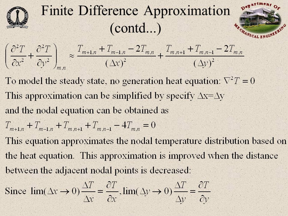
13. Finite Difference Approximation

14. Finite Difference Approximation (contd...)

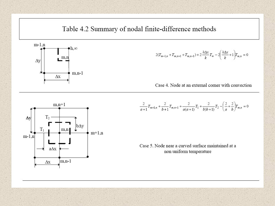
16. A System of Algebraic Equations  The nodal equations derived previously are valid for all interior points satisfying the steady state, no generation heat equation. For each node, there is one such equation. For example: for nodal point m=3, n=4, the equation is T 2,4 + T 4,4 + T 3,3 + T 3,5 - 4T 3,4 =0 T 3,4 =(1/4)(T 2,4 + T 4,4 + T 3,3 + T 3,5 )  Nodal relation table for exterior nodes (boundary conditions) can be found in standard heat transfer textbooks (Table 4.2 in this presentation).  Derive one equation for each nodal point (including both interior and exterior points) in the system of interest. The result is a system of N algebraic equations for a total of N nodal points.

19. Matrix Form A total of N algebraic equations for the N nodal points and the system can be expressed as a matrix formulation: [A][T]=[C]

20. Numerical Solutions  Matrix form: [A][T]=[C]. From linear algebra: [A] -1 [A][T]=[A] -1 [C], [T]=[A] -1 [C] where [A] -1 is the inverse of matrix [A]. [T] is the solution vector.  Matrix inversion requires cumbersome numerical computations and is not efficient if the order of the matrix is high (>10)

21. Numerical Solutions (contd…)  Gauss elimination method and other matrix solvers are usually available in many numerical solution package. For example, “Numerical Recipes” by Cambridge University Press or their web source at www.nr.com.  For high order matrix, iterative methods are usually more efficient. The famous Jacobi & Gauss-Seidel iteration methods will be introduced in the following.

22. Iteration Replace (k) by (k-1) for the Jacobi iteration

23. Iteration (contd…)  (k) - specify the level of the iteration, (k-1) means the present level and (k) represents the new level.  An initial guess (k=0) is needed to start the iteration.  By substituting iterated values at (k-1) into the equation, the new values at iteration (k) can be estimated  The iteration will be stopped when max  Ti (k) -Ti (k-1) , where  specifies a predetermined value of acceptable error