Download presentation
Presentation is loading. Please wait.

1
Analog Modulation - Why Modulation? Different analog modulation types
For each type:- - Mathematical presentation * Bandwidth * transmitted power - Modulators - Demodulators - Applications

2
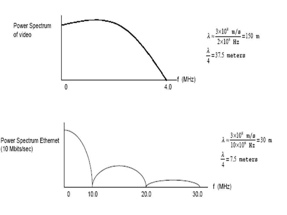
Why Modulation? Mainly for two reasons
1 - Practical antenna dimensions light velocity Wavelength frequency Dimension is in the order of a quarter wavelength

6
Why Modulation? 2- Multiplexing
Better utilization of the available frequency band Spectrum M3(f) M1(f) M2(f) MN(f) Frequency
 M1(f) M2(f) MN(f) Frequency.")
7
Basic Modulation Types
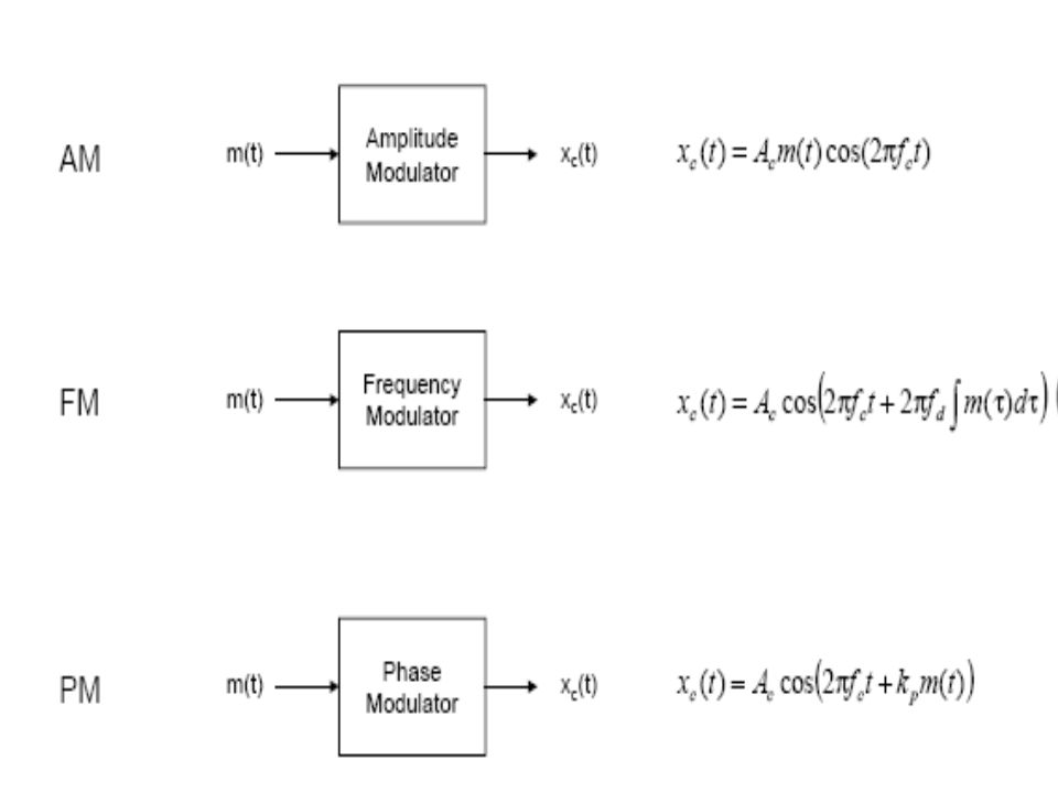
s (t) = A (t) cos [Ө (t) ] Ө (t) = ω t + φ (t) ‘ Ac cos ωc t ‘ is called unmodulated carrier Analog Modulation Digital Modulation
 = A (t) cos [Ө (t) ] Ө (t) = ω t + φ (t) ‘ Ac cos ωc t ‘ is called unmodulated carrier. Analog Modulation. Digital Modulation.")
8
Unmodulated carrier m(t) Modulator modulated signal: s(t)
Acos(2πfct+φ) modulated signal: s(t) Unmodulated carrier
 modulated signal: s(t) Unmodulated carrier.")
10
Modulation Types (Analog Modulation)
")
11
Modulation Types (Digital Modulation)
")
12
1- Amplitude Modulation (A.M) Conventional Amplitude Modulation
Consider a sinusoidal Carrier wave c(t) the unmodulated carrier. c(t) = Ac cos 2 π fc t Ac = carrier amplitude fc = carrier frequency A.M is the process in which the amplitude of the carrier wave c(t) is varied about a mean value, linearly with the base band signal
 the unmodulated carrier. c(t) = Ac cos 2 π fc t. Ac = carrier amplitude. fc = carrier frequency. A.M is the process in which the amplitude of the carrier wave c(t) is varied about a mean value, linearly with the base band signal.")
13
1-Amplitude Modulation
s(t) = Ac [1 + ka m(t) ] cos 2 π fc t = modulated signal where Ka = amplitude sensitivity [ volt]-1 s(t)= unmodulated carrier + upper side band + lower sideband s(t) = [ Ac + m(t)] cos 2 π fc t = Ac [ 1 + m(t) / Ac] cos 2 π fc t
 = Ac [1 + ka m(t) ] cos 2 π fc t. = modulated signal. where. Ka = amplitude sensitivity [ volt]-1. s(t)= unmodulated carrier + upper side band. + lower sideband. s(t) = [ Ac + m(t)] cos 2 π fc t. = Ac [ 1 + m(t) / Ac] cos 2 π fc t.")
14
1- Amplitude Modulation

15
1- Amplitude Modulation
The envelope has the same shape of m(t) as long as : І ka m(t) | < 1 for all values of ‘t’ This ensures that (1+ ka m(t)) is always positive i.e The modulation index less than 1 - percentage modulation is the modulation index multiplied by 100
 as long as : І ka m(t) | < 1 for all values of ‘t’ This ensures that (1+ ka m(t)) is always positive. i.e. - The modulation index less than 1. - percentage modulation is the modulation index multiplied by 100.")
16
1- Amplitude Modulation 100% modulation

17
1- Amplitude Modulation
Example: Let m(t) = Am cos 2 π fm t single tone signal Then s (t) = Ac [1 + μ cos 2 π fm t ] cos 2 π fc t μ = ka Am = modulation factor = modulation index μ x 100 = percentage modulation
 = Am cos 2 π fm t single tone signal. Then. s (t) = Ac [1 + μ cos 2 π fm t ] cos 2 π fc t. μ = ka Am. = modulation factor. = modulation index. μ x 100 = percentage modulation.")
18
1- Amplitude Modulation
-fc+fm -fc-fm fc f fc+fm fc-fm | S(f) | μAc/4 | M(f) | f fm -fm 1/2 | S(f) | | M(f) | -fc +fc -fm fm
 | μAc/4. | M(f) | f. fm. -fm. 1/2. | S(f) | | M(f) | -fc. +fc. -fm. fm.")
19
1- Amplitude Modulation
S(f) = (Ac/2) [ (f-fc) + (f-fc) ] + (Acμ/4) [ (f +(fc + fm)) ] + (Acμ/4) [ (f -(fc + fm)) ] + (Acμ/4) [ (f -(fc - fm)) ] + (Acμ/4) [ (f +(fc - fm)) ]
 = (Ac/2) [ (f-fc) + (f-fc) ] + (Acμ/4) [ (f +(fc + fm)) ] + (Acμ/4) [ (f -(fc + fm)) ] + (Acμ/4) [ (f -(fc - fm)) ] + (Acμ/4) [ (f +(fc - fm)) ]")
20
1- Amplitude Modulation
S(f)= (Ac/2) [ (f-fc) + (f-fc) ] + ( KaAc/2) [ M(f-fc) + M(f+fc)] U.S.B. is the upper side band L.S.B. is the lower side band B.W = 2W
= (Ac/2) [ (f-fc) + (f-fc) ] + ( KaAc/2) [ M(f-fc) + M(f+fc)] U.S.B. is the upper side band. L.S.B. is the lower side band. B.W = 2W.")
21
1- Amplitude Modulation
Unmodulated Power = carrier power= Ac2 / 2 U.S.B power = L.S.B. power = μ2 Ac2 / 8 Total side bands power = μ2 Ac2 / 4 Pt = Pc + Ps = (Ac2 / 2) + (μ2 Ac2 / 4) = Pc [ 1+ (μ2 /2) ] η = Side band power = μ2 total power μ2
 + (μ2 Ac2 / 4) = Pc [ 1+ (μ2 /2) ] η = Side band power = μ2. total power 2+ μ2.")
22
1- Amplitude Modulation
Computing percent of modulation from the modulation envelope .

23
1- Amplitude Modulation
Modulation by several sine waves The total modulation index is calculated by different methods one of them is the following:- If several sine waves modulate the carrier: The carrier power will be unaffected but the total side band power will be the sum of the individual side band powers

24
1- Amplitude Modulation
Pst = Ps Ps Ps3+. (Pcμt2 / 2) = (Pcμ12 / 2) + (Pcμ22 / 2)+ (Pcμ32 / 2) μt2 = μ12 + μ22 + μ32 +………… To calculate the total modulation index, take the square root of the sum of the squares of the individual modulation indices.
 = (Pcμ12 / 2) + (Pcμ22 / 2)+ (Pcμ32 / 2) μt2 = μ12 + μ22 + μ32 +………… To calculate the total modulation index, take the square root of the sum of the squares of the individual modulation indices.")
25
A.M. Modulators 1-Square Law Modulators
B.P.F cos2πfct m(t) ei eo vo A.M wave
 ei. eo. vo. A.M wave.")
26
A.M. Modulators 1-Square Law Modulators
For any non linear device e0 = an ein , taking the first two parts:- e0= a1ei + a2ei 2 e0= a1 [ m(t)+cos(2πfct)]+ a2[m(t)+ cos(2πfct)]2
+cos(2πfct)]+ a2[m(t)+ cos(2πfct)]2.")
27
1-Square Law Modulators
eo = a1m(t) + a2m2(t) +a1[1 + (2a2 / a1) m(t)] cos2πfct + (a2/2) [ 1+ cos4πfct] After B.P.F of B.W ‘W” centered at fc vo = a1[1 + (2a2 / a1) m(t)] cos2πfct Ac=a1 Ka = (2a2/ a1)
 + a2m2(t) +a1[1 + (2a2 / a1) m(t)] cos2πfct. + (a2/2) [ 1+ cos4πfct] After B.P.F of B.W ‘W centered at fc. vo = a1[1 + (2a2 / a1) m(t)] cos2πfct. Ac=a1 Ka = (2a2/ a1)")
28
2-Switching Modulator C(t) For І c(t) І >> , the diode acts as a switch. v1(t) = Ac cosωct + m(t) v2(t)= v1(t) for c(t) > 0 = 0 for c(t) < 0 Then v2(t)= [Ac cosωct + m(t)] gT0(t) v1 v2 B.P.F m(t) vA.M
= v1(t) for c(t) > 0. = 0 for c(t) < 0. Then v2(t)= [Ac cosωct + m(t)] gT0(t) v1. v2. B.P.F. m(t) vA.M.")
29
2-Switching Modulator Applying Fourrier series to gTo (t) we get:-
(1/2)+ (2/π) ((-1)n-1 / (2n-1)) cos[ωct(2n-1)] vA.M=(Ac/2) [ 1+(4/(πAc)) m(t) ] cos ωct Ka = 4 πAc
+ (2/π) ((-1)n-1 / (2n-1)) cos[ωct(2n-1)] vA.M=(Ac/2) [ 1+(4/(πAc)) m(t) ] cos ωct. Ka = 4. πAc.")
30
A.M.demodulator 1-Non coherent/ Asynchronous/Envelope Detector

31
Non-coherent demodulator

32
Non-coherent demodulator
The modulated signal is rectified by the diode and smoothed using the RC network For best operation The carrier frequency must be much higher than ‘W’. The discharge constant RC should be adjusted so that the maximum negative rate of the envelope will never exceed the exponential discharge. (1/W) > RC > Tc
 > RC > Tc.")
33
Amplitude Modulation Virtues, limitations and modifications of A.M.
Advantages: Ease of Modulation and demodulation ( cheap to build the system) Disadvantages - Wasteful of power. - Wasteful of B.W. We trade off system complexity to overcome these limitations - DSB-SC - DSB-QAM - SSB - VSB
 Disadvantages. - Wasteful of power. - Wasteful of B.W. We trade off system complexity to overcome these limitations. - DSB-SC - DSB-QAM. - SSB - VSB.")
34
2- Double Side bands Suppressed Carrier (DSB-SC)
The carrier component doesn’t appear in the modulated wave. s(t) = m(t) cos ( 2 πfct) S(f) = (1/2) [ M(f-fc) + M(f-fc) ] Total power = side bands power = (1/2) m2(t) B.W = 2W
 = m(t) cos ( 2 πfct) S(f) = (1/2) [ M(f-fc) + M(f-fc) ] Total power = side bands power = (1/2) m2(t) B.W = 2W.")
36
DSB-SC Modulators 1- Product Modulator
By multiplying the signal by any periodic waveform whose fundamental is ωc pT (t) = Pn exp (jnωct) m(t) pT (t) = Pn m(t) exp (jnωct) F {m(t) pT (t)} = Pn M(ω – ωc)
 = Pn exp (jnωct) m(t) pT (t) = Pn m(t) exp (jnωct) F {m(t) pT (t)} = Pn M(ω – ωc)")
37
DSB-SC Modulators x(t) m(t) x(t)= m(t) cos 2 π fc t cos 2 πfct
X(f) = (½)[ M(f+fc) + M(f-fc)] x(t) m(t) X cos 2 πfct
 = (½)[ M(f+fc) + M(f-fc)] x(t) m(t) X. cos 2 πfct.")
38
DSB-SC Modulators - + ~ 2- Using two square law modulators
cos 2 πfct m(t) m(t) cosωct +A c cosωct -m(t) cosωct +A c cosωct 2m(t) cosωct + - - m(t)
 m(t) cosωct +A c cosωct. -m(t) cosωct +A c cosωct. 2m(t) cosωct m(t)")
39
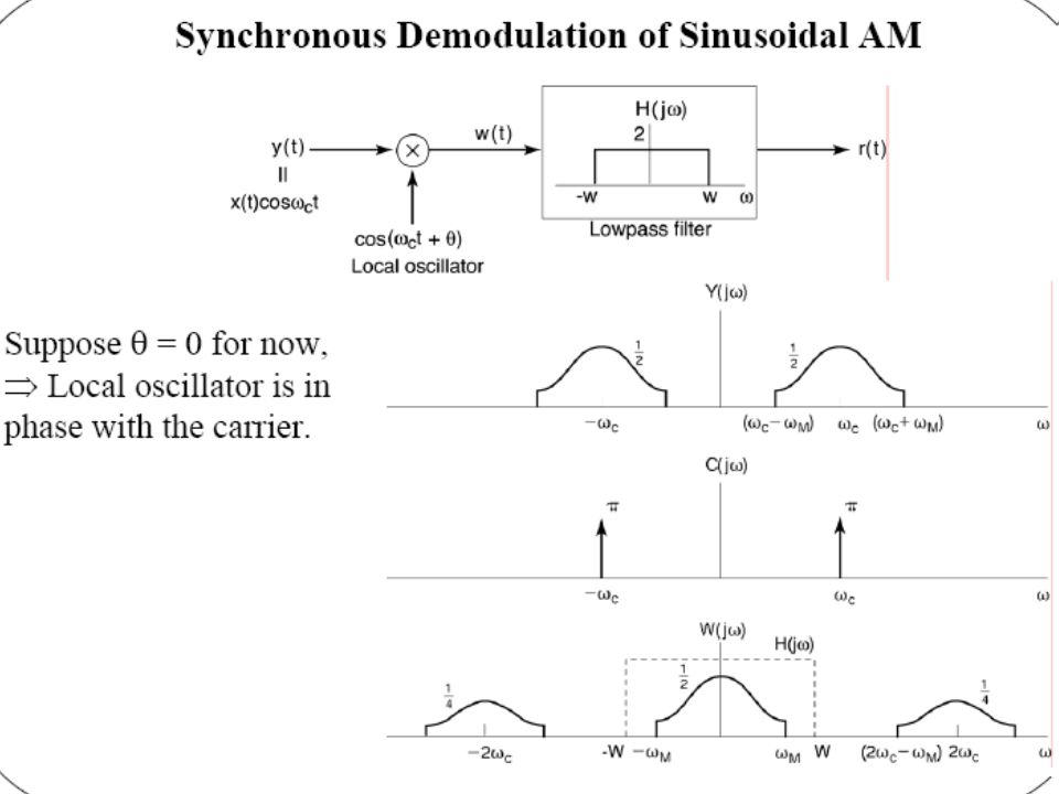
DSB-SC Demodulators Coherent (synchronous ) detection
Main problem : the carrier at the receiver must be synchronized in frequency and phase with the one at the transmitter. Otherwise we can have serious problems in the demodulation as will be seen.

41
DSB-SC Demodulators m(t) cosωct eo(t) ~ cos[ (ωc+ ∆ ω )t + φ]
X L.P.F ~ cos[ (ωc+ ∆ ω )t + φ] Frequency shift Phase shift
![DSB-SC Demodulators m(t) cosωct eo(t) ~ cos[ (ωc+ ∆ ω )t + φ]](http://slideplayer.com/slide/9523939/30/images/41/DSB-SC+Demodulators+m%28t%29+cos%CF%89ct+eo%28t%29+%7E+cos%5B+%28%CF%89c%2B+%E2%88%86+%CF%89+%29t+%2B+%CF%86%5D.jpg "X. L.P.F. ~ cos[ (ωc+ ∆ ω )t + φ] Frequency shift. Phase shift.")
42
DSB-SC Demodulators eo(t) = m(t) cos ωct cos[ (ωc+ ∆ ω )t + φ]
= (1/2) m(t) cos [ (∆ ω t) + φ] + cos [ (2 ωc +∆ ω) t + φ] Second term will be suppressed by the L.P.F. If ∆ ω =0 and φ = 0 eo(t) = (1/2) m(t) ( no frequency or phase error )
![DSB-SC Demodulators eo(t) = m(t) cos ωct cos[ (ωc+ ∆ ω )t + φ]](http://slideplayer.com/slide/9523939/30/images/42/DSB-SC+Demodulators+eo%28t%29+%3D+m%28t%29+cos+%CF%89ct+cos%5B+%28%CF%89c%2B+%E2%88%86+%CF%89+%29t+%2B+%CF%86%5D.jpg "= (1/2) m(t) cos [ (∆ ω t) + φ] + cos [ (2 ωc +∆ ω) t + φ] Second term will be suppressed by the L.P.F. If ∆ ω =0 and φ = 0. eo(t) = (1/2) m(t) ( no frequency or phase error )")
43
DSB-SC Demodulators If ∆ω=0 eo(t) = (1/2) m(t) cos φ
If φ = constant, eo(t) is proportional to m(t) Problems for φ either varying with time or equals to ± (π/2) The phase error may cause attenuation of the output signal without causing distortion as long as it is constant.
 is proportional to m(t) Problems for φ either varying with time or equals to ± (π/2) The phase error may cause attenuation of the output signal without causing distortion as long as it is constant.")
44
DSB-SC Demodulators If φ = 0 , ∆ω ≠ 0
eo(t) = (1/2) m(t) cos ∆ω t (Donald Duck) - The output is multiplied by a low frequency sinusoid, this causes attenuation and distortion of the output signal. - This could be solved by using detectors by square law device, or phase locked loops (PLL) (ex: Costas loop)
 = (1/2) m(t) cos ∆ω t (Donald Duck) - The output is multiplied by a low frequency sinusoid, this causes attenuation and distortion of the output signal. - This could be solved by using detectors by square law device, or phase locked loops (PLL) (ex: Costas loop)")
45
DSB-SC Demodulators Square law device The squared o/p = m2(t) cos2ωct
= (1/2)m2(t)+(1/2)m2(t)cos2ωct The N.B.F is tuned at the D.C component of m2(t) m(t) cos ωct S.L.D N.B.F(2fc) Freq div. by 2 L.P.F m(t)
m2(t)+(1/2)m2(t)cos2ωct. The N.B.F is tuned at the D.C component of m2(t) m(t) cos ωct. S.L.D. N.B.F(2fc) Freq div. by 2. L.P.F. m(t)")
46
DSB-SC Demodulators The B.P.F suppresses the m2(t) term.
After the frequency divider, the output = K cos ωct The synchronized carrier is generated spectrum 2fc f 2fc

47
DSB-SC Demodulators Costas Receiver Product modulator -90 phase shift
L.P.F V.C.O Phase Discriminator cos(2πfct+φ) Ac cos(2πfct)m(t) (1/2)Accos φ m(t) (1/2)Acsin φ m(t) K sin 2 φ
 Ac cos(2πfct)m(t) (1/2)Accos φ m(t) (1/2)Acsin φ m(t) K sin 2 φ.")
48
DSB-SC Demodulators The L.O. freq. is adjusted to be the same as fc
Suppose that the L.O. phase is the same as the carrier wave: ‘I’ o/p = m(t) ‘Q’ o/p = 0 Suppose that the L.O. phase drifts from its proper value by a small angle ‘φ’ radians. ‘I’ o/p will be the same and ‘Q’ o/p will be proportional to sin φ ~ φ (for small φ)
 ‘Q’ o/p = 0. Suppose that the L.O. phase drifts from its proper value by a small angle ‘φ’ radians. ‘I’ o/p will be the same and ‘Q’ o/p will be proportional to sin φ ~ φ (for small φ)")
49
DSB-SC Demodulators This ‘Q’ channel o/p will have the same polarity as the ‘I’ channel for one direction of L.O. phase drift and opposite polarity for the opposite direction of L.O. phase drift. By combining the ‘I’ and ‘Q’ channel ouputs in a phase discriminator (multiplier followed by L.P.F.) A d.c. control signal is obtained that automatically corrects for local phase error in the V.C.O.
 A d.c. control signal is obtained that automatically corrects for local phase error in the V.C.O.")
50
3- DSB quadruture carrier multiplexing (QAM)
It means quadruture amplitude modulation. We make use of the orthogonality of the sines and cosines to transmit and receive two different signals simultaneously on the same carrier frequency

51
3- DSB quadruture carrier multiplexing (QAM)
m1(t) x3 x1 X X L.P.F s(t) cosωct ~ + ~ cosωct + π/2 π/2 m2(t) x2 x4 X X L.P.F
 x3. x1. X. X. L.P.F. s(t) cosωct. ~ + ~ cosωct. + π/2. π/2. m2(t) x2. x4. X. X. L.P.F.")
52
3- DSB quadruture carrier multiplexing (QAM)
s(t) =m1(t) cos ωct + m2(t) sin ωct x1(t) = s(t) cos ωct = (1/2) m1(t)[1 + cos 2ωct ] + (1/2) m2(t) sin 2ωct x3(t) = (1/2) m1(t) x2(t) = s(t) sin ωct = (1/2) m2(t)[1 - cos 2ωct ] + (1/2) m1(t) sin 2ωct x4(t) = (1/2) m2(t)
 =m1(t) cos ωct + m2(t) sin ωct. x1(t) = s(t) cos ωct. = (1/2) m1(t)[1 + cos 2ωct ] + (1/2) m2(t) sin 2ωct. x3(t) = (1/2) m1(t) x2(t) = s(t) sin ωct. = (1/2) m2(t)[1 - cos 2ωct ] + (1/2) m1(t) sin 2ωct. x4(t) = (1/2) m2(t)")
53
4- Single Side Band (SSB)
Can be generated by: - Filter Method - Phase Shift Method Filter Method X S.B. Filter ~ m(t) s(t) S.S.B. Side band filter
 s(t) S.S.B. Side band filter.")
56
4- Single Side Band (SSB)
Phase shift method Hilbert transform. hilbert transform of s(t) |H(ω)| h(t) ω s(t) ӨH(ω) π/2 - π/2 ω
 |H(ω)| h(t) ω. s(t) ӨH(ω) π/2. - π/2. ω.")
57
4- Single Side Band (SSB)
It can be shown that:- s(t)S.S.B= m(t) cos ωct ± sin ωct X -π/2 cos ωct m(t) sin ωct m(t) cos ωct + sS.S.B
S.S.B= m(t) cos ωct ± sin ωct. X. -π/2. cos ωct. m(t) sin ωct. m(t) cos ωct. + sS.S.B.")
58
Detection of SSB Coherent Detection
y(t) = [ m(t) cos ωct ± sin ωct ] cos ωct = (1/2)m(t) [1+ cos 2ωct ] ± (1/2) sin 2 ωct After the L.P.F the output equals (1/2) m(t) Envelope Detection sS.S.B = R(t) cos [ωct + Ө(t)]
 = [ m(t) cos ωct ± sin ωct ] cos ωct. = (1/2)m(t) [1+ cos 2ωct ] ± (1/2) sin 2 ωct. After the L.P.F the output equals (1/2) m(t) Envelope Detection. sS.S.B = R(t) cos [ωct + Ө(t)]")
59
Detection of SSB R(t) = Ө(t) = tan-1 The envelope did’t express the signal but if we have large carrier in phase with the transmitted signal the non-coherent could be used. sS.S.B(t) + A cos ωct = R(t) cos [ωct + Ө(t)]
 + A cos ωct = R(t) cos [ωct + Ө(t)]")
60
Detection of SSB

61
Detection of SSB In case of large carrier, the envelope of
the S.S.B. signal has the form of m(t) (the base band signal), so the signal can be demodulated by the envelope detector with the condition that A >>> І m(t) І
 (the. base band signal), so the signal can be. demodulated by the envelope detector. with the condition that. A >>> І m(t) І.")
62
5- Vestigial Side Band (V.S.B)
Vestige means trace. Since S.S.B. is difficult to realize, a compromise between S.S.B. and D.S.B. in spectrum can be obtained using V.S.B. [especially when we have important components at low frequency and for large bandwidth base band signals like T.V.] Most of one side band is passed along with a vestige of the other side band. (B.W ~ W) (Reproduced by filters)
 (Reproduced by filters)")
63
5- Vestigial Side Band (V.S.B)
What is the shape of Hv(f)? X Hv(f) L.P.F A B C D E cos ωct
 X. Hv(f) L.P.F. A. B. C. D. E. cos ωct.")
64
5- Vestigial Side Band (V.S.B)
Spectrum at A prop. to: M(f) Spectrum at B prop. to: (1/2)[M(f+fc) + M(f-fc)] Spectrum at C prop. to: Hv(f)[M(f+fc) + M(f-fc)] Spectrum at D prop. to : (1/2) Hv(f+fc) [ M(f+2fc) + M(f) ] +(1/2) Hv(f-fc) [ M(f) + M(f-2fc) ] The central lobe of the spectrum at D must equal M(f) (1/2) [ Hv(f+fc) + Hv(f-fc) ] M(f) f f -fc fc
 Spectrum at B prop. to: (1/2)[M(f+fc) + M(f-fc)] Spectrum at C prop. to: Hv(f)[M(f+fc) + M(f-fc)] Spectrum at D prop. to : (1/2) Hv(f+fc) [ M(f+2fc) + M(f) ] +(1/2) Hv(f-fc) [ M(f) + M(f-2fc) ] The central lobe of the spectrum at D must equal M(f) (1/2) [ Hv(f+fc) + Hv(f-fc) ] M(f) f. f. -fc. fc.")
65
5- Vestigial Side Band (V.S.B)
What are the conditions on the vestigial filter? 1 – It must have an odd symmetry around fc 2 – 50% response level at fc [ Hv(f+fc) + Hv(f-fc) ] = constant in ‘W’ Hv(f) 1 1/2 -fc fc f
 + Hv(f-fc) ] = constant in ‘W’ Hv(f) 1. 1/2. -fc. fc. f.")
66
Comparison of Various AM signals
AM and AM_SC - Detectors required for AM are simpler - AM signals are easier to generate - SC requires less power at the transmitter for the same information ( cheaper transmitter) - Effect of fading is must serious in AM because the carrier must maintain a certain strenfth in relation to the side bands.
 - Effect of fading is must serious in AM because the carrier must maintain a certain strenfth in relation to the side bands.")
67
Comparison of Various AM signals
DSB and SSB - SSB needs only half the bandwidth - Fading disturbs the relationship of the two sidebands and causes more serious distortion than in the case of SSB,

68
AM Applications 1- Frequency Division Multiplexing (FDM)
If we have ‘N’ signals to be transmitted using AM modulation. All of these are band limited to ‘W’. A1 B1 C1 Mod 1 2 3 + f Dem A2 B2 C2 f1 f2 f3

69
Examples: radio, TV, telephone backbone, satellite, …

71
AM Applications Y(f) f f1 f2 B.P.F m1 2W at f1 Detector Carrier Demod.
~ mN Detector 2W at fN

72
AM Applications Example: Telephone channel multiplexing Basic Group 1
First Level Mux 1 2 12 Basic Group second 5 Super Group Third 10 Master Group North American FDM hierarchy

73
AM Applications All long-haul telephone channels are multiplexed by FDM using SSB. Basic Group consists of 12 FDM SSB voice signals each of BW = 4 KHz. It uses LSB spectra and occupies 60 to 108 KHz. [ alternate group configuration of 12 USB occupies 148 to 196 KHz] Basic group A (LSB)
")
74
AM Applications Basic Super group
consists of 60 channels. It is formed by multiplexing ‘5’ basic groups and it occupies a band of 312 to 552 KHz. [alternate 60 KHz to 300 KHz] Super group 1 (LSB)
")
75
AM Applications Basic master group
consiste of 600 channels. It is formed by multiplexing 10 supergroups.

76
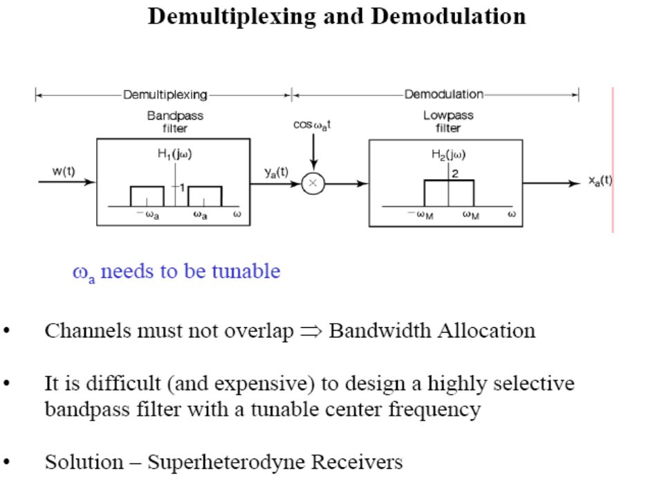
AM Applications 2- Superheterodyne receiver
The receiver not only has the task of demodulation but it is also required to perform some other tasks such as:- - Tuning : select the desired signal - Filtering : separate the desired signal from other modulated signals. - Amplification: to compensate for the loss in the signal power Superheterodyne receiver fulfils efficiently all the three functions

78
Basic elements of an AM receiver of the superheterodyne type
Mixer R.F. Section I.F. Section Envelop. detector A B C D ~ Local oscillator (fL.O) . Common tuning E Audio Amplifier
 . Common tuning. E. Audio Amplifier.")
79
Spectrum at different points
fc f I.F. response A.F. response fI.F R.F. response at ‘E’ at ‘C’ at ‘A’

80
at ‘A’: [A + m(t)] cos ωct
at ‘B’: [A1+a1m(t)] cos ωct cos (ωc + ωI.F)t [A2+a2m(t)] {cos (2ωc + ωI.F)t +cos ωI.Ft } at ‘C’: [A3+a3m(t)] cos ωI.Ft at ‘D’: a4m(t)
![at ‘A’: [A + m(t)] cos ωct](http://slideplayer.com/slide/9523939/30/images/80/at+%E2%80%98A%E2%80%99%3A+%5BA+%2B+m%28t%29%5D+cos+%CF%89ct.jpg "at ‘B’: [A1+a1m(t)] cos ωct cos (ωc + ωI.F)t. [A2+a2m(t)] {cos (2ωc + ωI.F)t +cos ωI.Ft } at ‘C’: [A3+a3m(t)] cos ωI.Ft. at ‘D’: a4m(t)")
81
The R. F cannot provide adequate selectivity since fc is high
The R.F cannot provide adequate selectivity since fc is high. It rejects a lot of adjacent channel interference and amplifies the signal. This is why we translate it to IF frequency to obtain good selectivity . All selectivity is realized in the IF section. The main role of RF section is image frequency rejection. What is the image frequency?

82
If fc = 1000 KHz , fL.O. = =1455KHz the image frequency = fc+2fI.F.= 1910 KHz. Will also be picked up. Stations that are 2fI.F apart are called image stations and are rejected by RF filter. Up-conversion: fL.O. = fc+fI.F Down conversion: fL.O= fc-fI.F

Similar presentations


 Carrier Wave Modulation Systems.>")


>")


 TV (0-6 MHz) A signal may be sent in its baseband.>")
 is transformed Into waveforms that are.>")
>")
