1. Stat 112 Notes 6 Today: –Chapters 4.2 (Inferences from a Multiple Regression Analysis)

2. Multiple Linear Regression Model

4. Predicted Values and Residuals Predicted Value for Observation with Residual for observation i = prediction error for observation i = Obtaining the predicting values and residuals in JMP: After using Fit Model to fit the multiple regression model, click the red triangle next to Response, click Save Columns and then click Predicted Values and Residuals. Columns with the predicted values and residuals will be created.

5. Cars that Have Unexpected Gas Mileage Given Their Weight, Horsepower, Cargo and Seating Gas guzzlers (highest residuals): 1. Mercedes Benz G500: 12.04 2. Chevrolet Tracker: 9.12 3. Jeep Wrangler SE: 8.39 Environment friendly (most negative residuals): 1.Volkwagen Phaeton: -7.96 2.BMW 745i: -7.75 3.Toyota Scion xA: -6.03

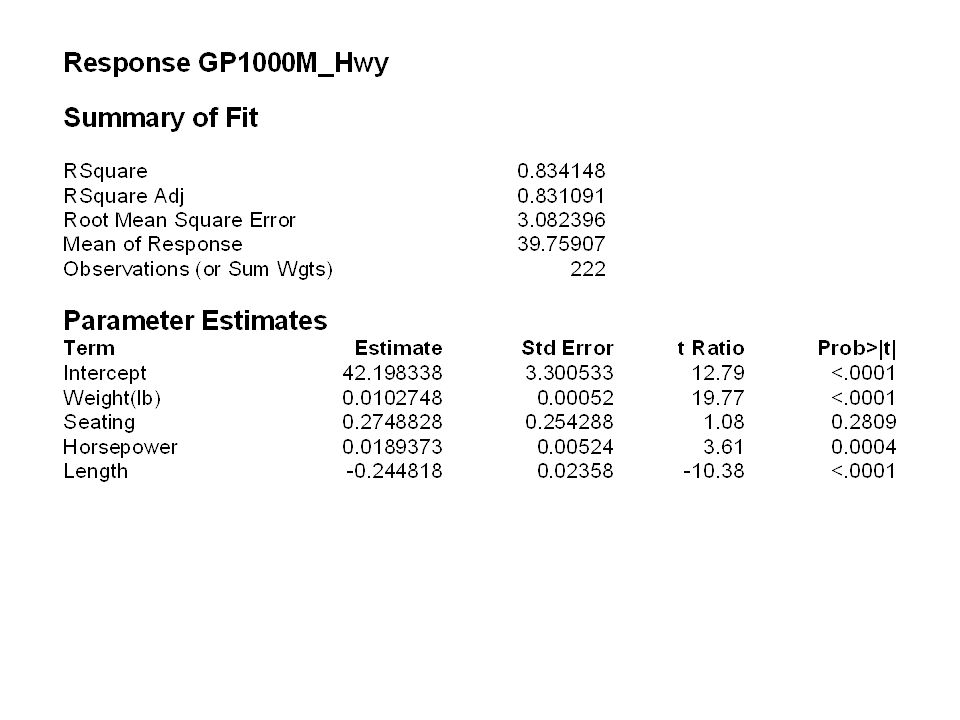
6. Interpretation of Regression Coefficients Gas mileage regression from car04.JMP

7. Partial Slopes vs. Marginal Slopes Multiple Linear Regression Model: The coefficient is a partial slope. It indicates the change in the mean of y that is associated with a one unit increase in while holding all other variables fixed. A marginal slope is obtained when we perform a simple regression with only one X, ignoring all other variables. Consequently the other variables are not held fixed.

8. Path Diagram X1X1 X2X2 Y

9. Partial vs. Marginal Slopes Example

10. Partial and Marginal Slopes of Length

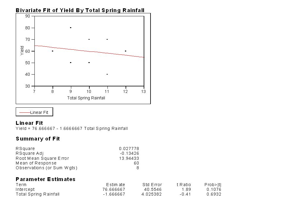
11. Partial Slopes vs. Marginal Slopes: Another Example In order to evaluate the benefits of a proposed irrigation scheme in a certain region, suppose that the relation of yield Y to rainfall R is investigated over several years. Data is in rainfall.JMP.

13. Higher rainfall is associated with lower temperature.

14. Rainfall is estimated to be beneficial once temperature is held fixed. Multiple regression provides a better picture of the benefits of an irrigation scheme because temperature would be held fixed in an irrigation scheme.

15. Path Diagram Rainfall Temperature Yield 5.71 -2.5 2.95

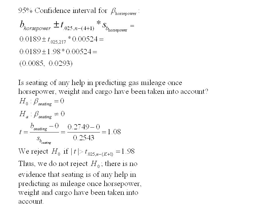
16. Inferences about Regression Coefficients Confidence intervals: confidence interval for : Degrees of freedom for t equals n-(K+1). Standard error of,, found on JMP output. Hypothesis Test: Decision rule for test: Reject H 0 if or where p-value for testing vs. is printed in JMP output under Prob>|t|.

17. Inference Examples Find a 95% confidence interval for ? Is seating of any help in predicting gas mileage once weight, horsepower and length have been taken into account? Carry out a test at the 0.05 significance level.

19. Checking the Assumptions

20. Plots for Checking Assumptions We can construct residual plots of each explanatory variable X k vs. the residuals. We save the residuals by clicking the red triangle next to Response after fitting the model and clicking Save Columns and then residuals. We then plot X k vs. the residuals using Fit Y by X (where Y=the residuals). We can plot a horizontal line at 0 by using Fit Y by X (it is a property of multiple linear regression that the least squares line for the regression of the residuals on any X k is a horizontal line. A useful summary of the residual plots for each explanatory variable is the Residual by Predicted plot that is automatically plotted after using Fit Model. The residual by predicted plot is a plot of the predicted values,, vs. the residuals

21. Checking Assumptions Linearity: –Check that in residual by predicted plot, the mean of the residuals for each range of the predicted values is about zero. –Check that in each residual plot, the mean of the residuals for each range of the explanatory variable is about zero. Constant Variance: Check that in the residual by predicted plot that for each range of the predicted values, the spread of the residuals is about the same. Normality: Make normal quantile plot of the residuals. Check that all the residuals are inside of the two confidence bands.

22. Residual by predicted plot suggests linearity and constant variance assumptions are okay. Plot of weight vs. residuals suggests linearity is okay. Plot of horsepower vs. residuals suggests linearity is okay.

23. Plot of residuals vs. seating suggests linearity is not perfect for seating. Residuals for small and high seating seem to have a mean that is smaller than 0. Plot of residuals vs. horsepower suggest linearity is okay.

24. Checking Normality There is a slight violation of normality. A few points are outside the lower confidence bound. We will discuss how to address violations of normality later in the course.

25. R-Squared (Coefficient of Determination) The coefficient of determination for multiple regression is defined as for simple linear regression: Represents percentage of variation in y that is explained by the multiple regression line. is between 0 and 1. The closer to 1, the better the fit of the regression equation to the data. For the gas mileage regression, RSquare0.834148 Summary of Fit