Download presentation
Presentation is loading. Please wait.

1
Klein-Gordon Equation in the Gravitational Field of a Charged Point Source D.A. Georgieva, S.V. Dimitrov, P.P. Fiziev, T.L. Boyadjiev Gravity, Astrophysics and Strings, Kiten’ 05

2
We solve a problem of motion of a neutral point particle in the gravitational field in the background of a charged point-like source.

3
A point particle solution of Einstein-Maxwell field equations has the form: where luminosity variable, radial coordinate when where finite luminosity of the point source

4
We use the metric coefficient g as an independent variable instead of the radial coordinate or luminosity variable. This gives the following dependence of the luminosity variable on g: with where classical radius,the parameter connects the classical radius with the Schwarzschild radius via

5
The wave functionof a massive non-charged scalar field interacting in the gravitational field (1) of a point-like source satisfies the following Klein-Gordon equation: is the D’Alambert operator. in case of spherical symmetry, described by metric (1). angular part of the Laplace- Beltrami operator. Then, in case of spherical symmetry the KGE has the form:
. angular part of the Laplace- Beltrami operator. Then, in case of spherical symmetry the KGE has the form:.")
6
The angular part of the wave function can be explicitly derived in terms of spherical harmonics eigenfunctions of the angular part of the Laplace- Beltrami operator, i.e. Separation of variables Then, for the wave functionwe obtain the equation

7
Due to invariance with respect to time translations one has: so that the radial function is a solution of a second order Ordinary Differential Equation – the radial KGE: Substitutingwe get The final form of KGE

8
We change the variables with the tortoise coordinate u is a dimensionless tortoise variable. From formula (2) we get for g(u) : Introducing becomes (dimensionless) the KGE with a potential (3)
 we get for g(u) : Introducing becomes (dimensionless) the KGE with a potential (3).")
9
g(u 0 ) k The function g(u) is implicitly defined as a solution of the following Cauchy problem: where u 0 is an arbitrary constant and k is the gravitational mass defect of the point source. The function g(u) can be given implicitly by: g(u): u u 0 F (g) – F ( k ). The function F(g) depends on the values of
 can be given implicitly by: g(u): u u 0 F (g) – F ( k ). The function F(g) depends on the values of .")
10
Case The Cauchy problem has two singular points: at g (regular) and (irregular). Case There are two irregular singularities: g and g .

11
Case > 1: In this case one has three singular points g , g and g . The first two are regular. They corresponds to the event horizon M and the classical radius Q / M respectively. The singular point g is essentially irregular and corresponds to and g must satisfy:

12
The general solution of equation (3) depends on two arbitrary constants and the eigenvalue , P l (u) = P l (u;C 1 ;C 2 ; ). These three parameters can be defined from the boundary conditions for the problem and the normalization condition that the wave function satisfies. - the wave function is zero at the place where the source is positioned. - Comes from the asymptotic behavior at infinity. - L 2 normalization condition.

13
g(u 0 ) k
 k ")
14
We use a algorithm based on the Continuous Analogue of Newton’s Method. Let y note the couple (P l (u), ), where . 1) – we introduce a formal evolution parameter i.e. we mark 2) – we suppose thatand whenwhere y 0 is a given initial approximation sufficiently close to the exact solution
, ), where . 1) – we introduce a formal evolution parameter i.e. we mark 2) – we suppose thatand whenwhere y 0 is a given initial approximation sufficiently close to the exact solution.")
15
3) – let us put where dot denotes the derivative by t. 4) – applying CANM to the spectral problem we obtain the following system for Z(u) and (4)
 – applying CANM to the spectral problem we obtain the following system for Z(u) and (4).")
16
5) – the solution of the problem (4) is sought in the form: where v(u) is a new unknown function. Substituting the expansion for Z (u) in (4) we get that v(u) is a solution of the linear boundary value problem: 6) – if we know v(u) the quantity can be calculated from the equality (5)
 in (4) we get that v(u) is a solution of the linear boundary value problem: 6) – if we know v(u) the quantity can be calculated from the equality (5).")
17
7) – if y 0 is a given initial approximation, at each iteration k = 0,1, 2,... the next approximation to the exact solution is obtained by formulas – a given discretization of “time” t. 8) – the linear boundary value problems (5) are solved at each step using a hermitian spline-collocation scheme of fourth order of approximation.
 – the linear boundary value problems (5) are solved at each step using a hermitian spline-collocation scheme of fourth order of approximation..")
19
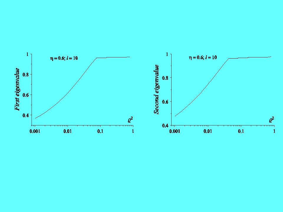
Case: < 1

22
1) – We solved numerically the problem of a motion of a neutral point particle in gravitational field in the background of a charged point-like source. 2) – The new boundary conditions determine a new spectrum similar to the spectrum in the case of motion of a particle in the gravitational field of a non-charged source.
 – The new boundary conditions determine a new spectrum similar to the spectrum in the case of motion of a particle in the gravitational field of a non-charged source..")
Similar presentations


 arises in a low-energy asymptotic of string theory models and in certain.>")


