1. Slide 1 © 2011 Cengage Learning. All Rights Reserved. May not be scanned, copied or duplicated, or posted to a publicly accessible website, in whole or in part. Business and Economic Forecasting Business and Economic Forecasting is a critical managerial activity which comes in many forms including: l Quantitative Forecasting +2.17% Gives the precise amount or percentage Qualitative Forecasting Qualitative Forecasting Gives the expected direction Up, down, or about the same

2. Slide 2 The Significance of Forecasting Both public and private enterprises operate under conditions of uncertainty. Management wishes to limit this uncertainty by predicting changes in cost, price, sales, and interest rates. Accurate forecasting can help develop strategies to promote profitable trends and to avoid unprofitable ones. A forecast is a prediction concerning the future. Good forecasting will reduce, but not eliminate, the uncertainty that all managers feel.

3. Slide 3 Hierarchy of Forecasts The selection of forecasting techniques depends in part on the level of economic aggregation involved. The hierarchy of forecasting is: National Economy (GDP, interest rates, inflation, etc.) »Sectors of the economy (durable goods)  Industry forecasts (all automobile manufacturers)  Firm forecasts (Ford Motor Company) oProduct forecasts (The Ford Focus)

4. Slide 4 Criteria Used to Select a Technique The choice of a particular forecasting method depends on several criteria: 1. costs of the forecasting method compared with its gains 2. complexity of the relationships among variables 3. time period involved 4. lead time between receiving information and the decision to be made 5. accuracy of the forecast

5. Slide 5 Accuracy of Forecasting The accuracy of a forecasting model is measured by how close the actual variable, Y, ends up to the forecasting variable,. Forecast error is the difference. (Y - ) Models differ in accuracy, which is often based on the square root of the average squared forecast error over a series of N forecasts and actual figures Called a root mean square error, RMSE:

6. Slide 6 ALTERNATIVE FORECASTING TECHNIQUES Alternative forecasting techniques can be classified in the following general categories: »Deterministic trend analysis »Smoothing techniques »Barometric indicators »Survey and opinion-polling techniques »Macroeconometric models

7. Slide 7 Deterministic Trend Analysis Time-series data. A series of observations taken on an economic variable at various past points in time. »Secular trends »Cyclical variations »Seasonal effects »Random fluctuations Cross-sectional data. Series of observations taken on different observation units (for example, households, states, or countries) at the same point in time. »Ratio to trend method »Dummy variables

8. Slide 8 FIGURE 5.2 Secular, Cyclical, Seasonal, and Random Fluctuations in Time Series Data

9. Slide 9 FIGURE 5.2 Secular, Cyclical, Seasonal, and Random Fluctuations in Time Series Data

10. Slide 10 Elementary Time Series Models for Economic Forecasting Y t+1 = Y t »The simplest method »Best when there is no trend, only random error »Graphs of sales over time with and without trends »When trending down, the simplest predicts too high NO Trend Trend          ^ time

11. Slide 11

12. Slide 12 Secular Trends Y t+1 = Y t + (Y t - Y t-1 ) »This equation begins with last period’s forecast, Y t, just like the simple forecast. »Plus an ‘adjustment’ for the change in the amount between periods Y t and Y t-1. »When the forecast is trending up or down, this adjustment works better than the simple forecast method #1. ^

13. Slide 13 Deterministic Trend Analysis Components of Time Series TIME T0T0 X X X Dependent Variable Forecasted Amounts The data may offer secular trends, cyclical variations, seasonal variations, and random fluctuations.

14. Slide 14 Time Series Examine Patterns in the Past TIME T0T0 X X X Dependent Variable Secular Trend Forecasted Amounts The data may offer secular trends, cyclical variations, seasonal variations, and random fluctuations.

15. Slide 15 Time Series Examine Patterns in the Past TIME T0T0 X X X Dependent Variable Secular Trend Cyclical and Seasonal Variation Forecasted Amounts The data may offer secular trends, cyclical variations, seasonal variations, and random fluctuations.

16. Slide 16 Linear Trend & Constant Rate of Growth Trend Used when trend has a constant AMOUNT of change Y t = a + bT, where t Y t are the actual observations and T T is a numerical time variable Used when trend is a constant PERCENTAGE rate Log Y t = a + bT, b where b is the continuously compounded growth rate Linear Trend Growth Uses a Semi-log Regression

17. Slide 17 FIGURE 5.4 Prizer Creamery: Monthly Ice Cream Sales

18. Slide 18 More on Constant Rate of Growth Model – a proof Suppose: Y t = Y 0 ( 1 + g) t where g is the annual growth rate Take the natural log of both sides: »Ln Y t = Ln Y 0 + t Ln (1 + g) »but Ln ( 1 + g )  g, the continuously compounded growth rate »SO: Ln Y t = Ln Y 0 + t g Ln Y t =  +  t where  is the growth rate, g. ^ ^

19. Slide 19 Numerical Examples: 6 observations MTB > Print c1-c3. Sales Time Ln-sales 100.0 1 4.60517 109.8 2 4.69866 121.6 3 4.80074 133.7 4 4.89560 146.2 5 4.98498 164.3 6 5.10169 Using this sales data, estimate sales in period 7 using a linear and a semi-log functional form

20. Slide 20 The linear regression equation is Sales = 85.0 + 12.7 Time Predictor Coef Stdev t-ratio p Constant 84.987 2.417 35.16 0.000 Time 12.6514 0.6207 20.38 0.000 s = 2.596 R-sq = 99.0% R-sq(adj) = 98.8% The semi-log regression equation is Ln-sales = 4.50 + 0.0982 Time Predictor Coef Stdev t-ratio p Constant 4.50416 0.00642 701.35 0.000 Time 0.098183 0.001649 59.54 0.000 s = 0.006899 R-sq = 99.9% R-sq(adj) = 99.9%

21. Slide 21 Forecasted Sales @ Time = 7 Linear Model Sales = 85.0 + 12.7 Time Sales = 85.0 + 12.7 ( 7) Sales = 173.9 Semi-Log Model Ln-sales = 4.50 + 0.0982 Time Ln-sales = 4.50 + 0.0982 ( 7 ) Ln-sales = 5.1874 To anti-log: »e 5.1874 = 179.0  linear 

22. Slide 22 Sales Time Ln-sales 100.0 1 4.60517 109.8 2 4.69866 121.6 3 4.80074 133.7 4 4.89560 146.2 5 4.98498 164.3 6 5.10169 179.07 semi-log 173.97 linear Which prediction do you prefer? Semi-log is exponential 7

23. Slide 23 Declining Rate of Growth Trend A number of marketing penetration models use a slight modification of the constant rate of growth model In this form, the inverse of time is used Ln Y t =  1 –  2 ( 1/t ) This form is good for patterns like the one to the right It grows, but at continuously a declining rate time Y

24. Slide 24 Seasonal Adjustments: The Ratio to Trend Method Take ratios of the actual (A) to the forecasted (F) values for past years. A 1 /F 1, A 2 /F 2, A 3 /F 3, find average of these ratios. This is the seasonal adjustment Adjust by this percentage by multiply your forecast by the seasonal adjustment »If average ratio is 1.02, adjust forecast upward 2% 12 quarters of data 1 2 3 4 1 2 3 4 1 2 3 4            

25. Slide 25 Let D = 1, if 4th quarter and 0 otherwise Run a new regression: Y t = a + bT + cD »the “c” coefficient gives the amount of the adjustment for the fourth quarter. It is an Intercept Shifter. »With 4 quarters, there can be as many as three dummy variables; with 12 months, there can be as many as 11 dummy variables EXAMPLE: Sales = 300 + 10T + 18D 12 Observations from the first quarter of 2008-I to 2010-IV. Forecast all of 2011. Sales(2011-I) = 430; Sales(2011-II) = 440; Sales(2011-III) = 450; Sales(2011-IV) = 478 Seasonal Adjustments: Dummy Variables

26. Slide 26 Smoothing Techniques: Moving Averages A smoothing forecast method for data that jumps around Best when there is no trend 3-Period Moving Ave is: Y t+1 = [Y t + Y t-1 + Y t-2 ]/3 For more periods, add them up and take the average * * * * * Forecast Line is Smoother TIME Dependent Variable ^

27. Slide 27 FIGURE 5.6 Walker Corporation’s Three- Month Moving Average Sales Forecast Chart

28. Slide 28 Smoothing Techniques First-Order Exponential Smoothing A hybrid of the Naive and Moving Average methods Y t+1 = wY t +(1-w)Y t A weighted average of past actual and past forecast, with a weight of w Each forecast is a function of all past observations Can show that forecast is based on geometrically declining weights. Y t+1 = w Y t +(1-w)wY t-1 + (1-w) 2wY t-2 + … Find lowest RMSE to pick the best w. ^ ^ ^

29. Slide 29 First-Order Exponential Smoothing Example for w =.50 Actual SalesForecast 100100initial seed required 120.5(100) +.5(100) = 100 115 130 ? 1234512345

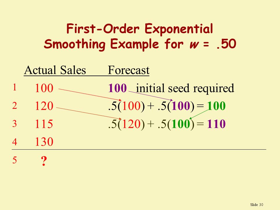
30. Slide 30 First-Order Exponential Smoothing Example for w =.50 Actual SalesForecast 100100initial seed required 120.5(100) +.5(100) = 100 115.5(120) +.5(100) = 110 130 ? 1234512345

31. Slide 31 First-Order Exponential Smoothing Example for w =.50 Actual SalesForecast 100100initial seed required 120.5(100) +.5(100) = 100 115.5(120) +.5(100) = 110 130.5(115) +.5(110) = 112.50 ?.5(130) +.5(112.50) = 121.25 Period 5 Forecast MSE = {(120-100) 2 + (110-115) 2 + (130-112.5) 2 }/3 = 243.75 RMSE =  243.75 = 15.61 1234512345

32. Slide 32 Barometric Techniques

33. Slide 33 Barometric Techniques

34. Slide 34 Direction of sales can be indicated by other variables. TIME Index of Capital Goods peak PEAK Motor Control Sales 4 Months Example: Index of Capital Goods is a “leading indicator” There are also lagging indicators and coincident indicators Barometric Techniques

35. Slide 35 LEADING INDICATORS* »M2 money supply (-14.2) »S&P 500 stock prices (-11.1) »Building permits (-15.4) »Initial unemployment claims (-12.9) »Contracts and orders for plant and equipment (-7.3) COINCIDENT INDICATORS »Nonagricultural payrolls (+.8) »Index of industrial production (-1.1) »Personal income less transfer payment (-.4) LAGGING INDICATORS »Inventory to sales ratio (9.2) »Prime rate (+2.0) »Change in labor cost per unit of output (+6.4) *http://www.nber.org Average time given in months from reference peaks Table 5.7

36. Slide 36 Surveys and Opinion Polling Techniques New product ideas have no historical data, but surveys can assess interest ( Would you buy a phone that is also a Swiss knife? ) Macroeconomic surveys include: »Plant and equipment expenditure plans (McGraw-Hill, National Industrial Conference Board, US Department of Commerce, Fortune). »Plans for inventory changes and sales expectations (US Department of Commerce, McGraw-Hill, Dun and Bradstreet, and the National Association of Purchasing Agents) »Consumer expenditure plans (U of Michigan’s Survey Research Center on plans to buy autos, called consumer sentiment) Sales Forecasting include: »Sales force polling (sales people know what their customers are saying) »Surveys of consumer intentions (asking prior customer’s their intentions for replacing appliances, windows, etc.)

37. Slide 37 Econometric Models Single Equation Models Specify the variables in the model. One example is attendance at NFL games involving 14 variables from price, weather, domes, non-Sunday games, and winning record at home. Estimate the parameters of a typical demand function: »Q d = a + bP + cI + dP s + eP c But forecasts require estimates for future prices, future income, etc. Often combine econometric models with time series estimates of the independent variable.

38. Slide 38 Q d = 400 -.5P + 2Y +.2P s »anticipate pricing the good at P = $20 »Income (Y) is growing over time, the estimate is: Ln Y t = 2.4 +.03T, and next period is T = 17. Y = e 2.910 = 18.357 »The prices of substitutes are likely to be P = $18. Find Q d by substituting in predictions for P, Y, and P s Hence Q d = 430.31

39. Slide 39 Econometric Models Multi-Equation Models In market (and life) interrelationships may be complex. Macroeconomic models of national income often involve several equations for consumption, GDP, investment and government. i.C =  1 +  1 (GDP – T) +  1 ii.I =  2 +  2 P t-1 +  2 iii.T =  3 GDP +  3 iv.GDP = C + I + G Such models offer forecasts, but can be supplemented with judgment of the forecasters.

40. Slide 40

41. Slide 41