2. Recap Functions with No input OR No output Determining The Number of Input and Output Arguments Local Variables Global Variables Creating ToolBox of Functions Anonymous Functions and Function Handles Function Functions Subfunctions

3. Summary of Chapter MATLAB contains a wide variety of built-in functions However, you will often find it useful to create your own MATLAB functions The most common type of user-defined MATLAB function is the function M-file, which must start with a function-definition line that contains the word function a variable that defines the function output a function name a variable used for the input argument For example, function output = my_function(x)

4. Continued…. The function name must also be the name of the M-file in which the function is stored Function names follow the standard MATLAB naming rules Like the built-in functions, user-defined functions can accept multiple inputs and can return multiple results Comments immediately following the function-definition line can be accessed from the command window with the help command Variables defined within a function are local to that function. They are not stored in the workspace and cannot be accessed from the command window Global variables can be defined with the global command used in both the command window and a MATLAB function. Good programming style suggests that define global variables with capital letters. In general, however, it is not wise to use global variables

5. Continued…. Groups of user-defined functions, called “toolboxes,” may be stored in a common directory and accessed by modifying the MATLAB® search path. This is accomplished interactively with the path tool, either from the menu bar, as in File -> Set Path or from the command line, with pathtool MATLAB provides access to numerous toolboxes developed at The MathWorks or by the user community Another type of function is the anonymous function, which is defined in a MATLAB session or in a script M-file and exists only during that session Anonymous functions are especially useful for very simple mathematical expressions or as input to the more complicated function functions

6. Chapter 13 Numerical Techniques

7. Introduction Interpolate between data points, using either linear or cubic spline models Model a set of data points as a polynomial Use the basic fitting tool Use the curve-fitting toolbox Perform numerical differentiations Perform numerical integrations Solve differential equations numerically

8. Interpolation Especially when we measure things, we don’t gather data at every possible data point Consider a set of x–y data collected during an experiment By using an interpolation technique, we can estimate the value of y at values of x where we didn’t take measurement The two most common interpolation techniques are Linear interpolation Cubic spline interpolation both of which are supported by MATLAB

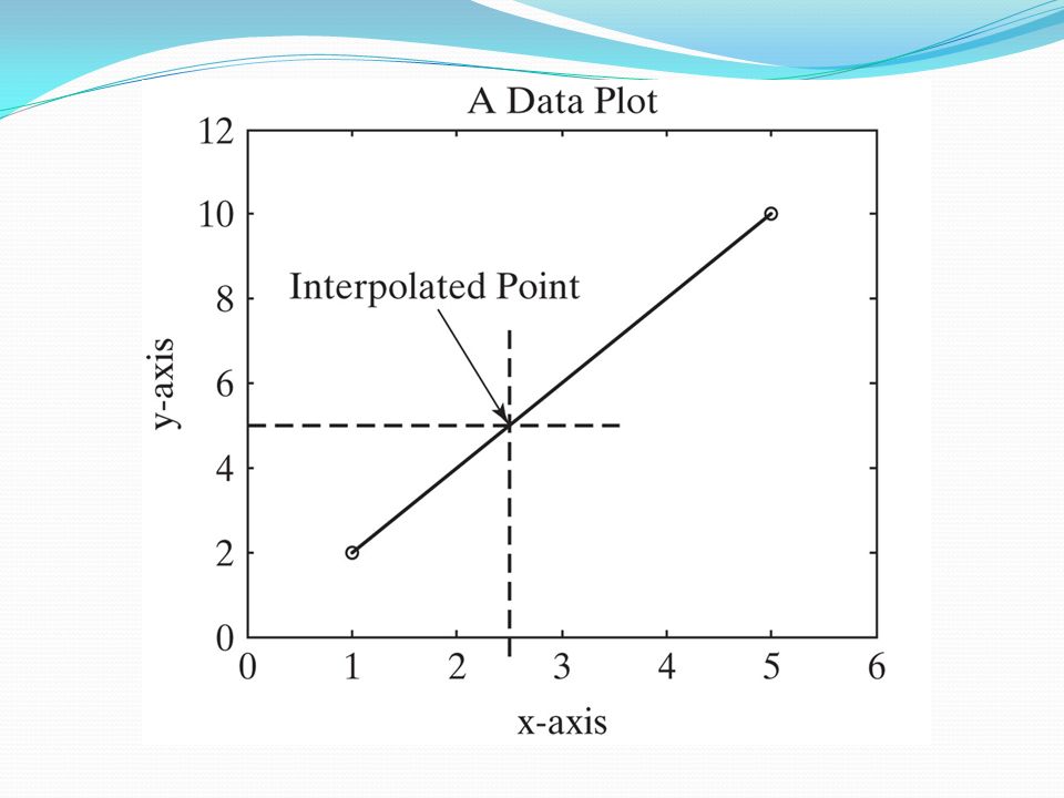
9. Interpolation between data points

10. Linear Interpolation The most common way to estimate a data point between two known points is linear interpolation In this technique, we assume that the function between the points can be estimated by a straight line drawn between them If we find the equation of a straight line defined by the two known points, we can find y for any value of x The closer together the points are, the more accurate our approximation is likely to be

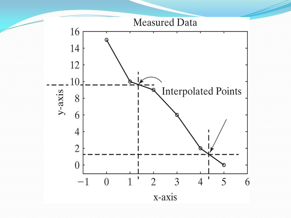
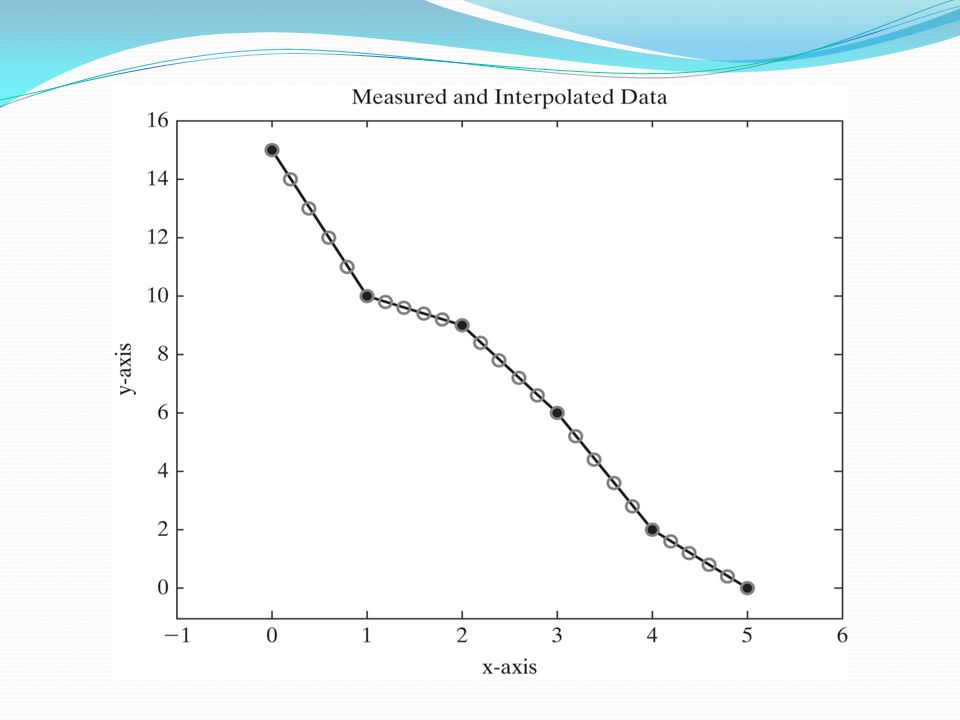
12. Continued…. We can perform linear interpolation in MATLAB with the interp1 function We’ll first need to create a set of ordered pairs to use as input to the function The data used to create the right-hand graph of next figure is x = 0:5; y = [15, 10, 9, 6, 2, 0];

14. Continued…. To perform a single interpolation, the input to interp1 is the x data, the y data, and the new x value for which you’d like an estimate of y For example: to estimate the value of y when x is equal to 3.5, type interp1(x,y,3.5) ans = 4 You can perform multiple interpolations all at the same time by putting a vector of x -values in the third field of the interp1 function For example: to estimate y -values for new x ’s spaced evenly from 0 to 5 by 0.2, type new_x = 0:0.2:5; new_y = interp1(x,y,new_x) which returns new_y = Columns 1 through 5 15.0000 14.0000 13.0000 12.0000 11.0000 Columns 6 through 10 10.0000 9.8000 9.6000 9.4000 9.2000 Columns 11 through 15 9.0000 8.4000 7.8000 7.2000 6.6000 Columns 16 through 20 6.0000 5.2000 4.4000 3.6000 2.8000 Columns 21 through 25 2.0000 1.6000 1.2000 0.8000 0.4000 Column 26 0 Graph is plotted as plot(x,y,new_x,new_y,'o')

16. Continued…. The interp1 function defaults to linear interpolation to make its estimates. However, other approaches are possible If we want (probably for documentation purposes) to explicitly define the approach used in interp1 as linear interpolation, we can specify it in a fourth field: interp1(x, y, 3.5, 'linear') ans = 4