1. Lecture 3 : Isosurface Extraction

2. Isosurface Definition  Isosurface (i.e. Level Set ) :  Constant density surface from a 3D array of data  C(w) = { x | F(x) - w = 0 } ( w : isovalue, F(x) : real-valued function, usually 3D volume data ) isosurfacing

3. Isosurface Triangulation Idea: –create a triangular mesh that will approximate the iso-surface –calculate the normals to the surface at each vertex of the triangle Algorithm: –locate the surface in a cube of eight pixels –calculate vertices/normals and connectivity –march to the next cube

4. Marching Cubes [Lorensen and Cline, ACM SIGGRAPH ’87] Goal –Input : 2D/3D/4D imaging data (scalar) –Interactive parameter : isovalue selection –Output : Isosurface triangulation isosurfacing

5. Isosurface Extraction 2. Isocontouring [Lorensen and Cline87,…] Definition of isosurface C(w) of a scalar field F(x) C(w)={x|F(x)-w=0}, ( w is isovalue and x is domain R 3 ) ( Isocontour in 2D function: isovalue=0.5 ) Marching Cubes for Isosurface Extraction 1.Dividing the volume into a set of cubes 2.For each cubes, triangulate it based on the 2^8(reduced to 15) cases 0.70.60.750.4 0.80.40.6 0.4 0.3 0.35 0.25 1.0 0.80.40.3 0.70.60.750.4 0.80.40.6 0.4 0.3 0.35 0.25 1.0 0.80.40.3 0.70.60.750.4 0.80.40.6 0.4 0.3 0.35 0.25 1.0 0.80.40.3

6. Surface Intersection in a Cube assign ZERO to vertex outside the surface assign ONE to vertex inside the surface Note: –Surface intersects those cube edges where one vertex is outside and the other inside the surface

7. Surface Intersection in a Cube There are 2^2=256 ways the surface may intersect the cube Triangulate each case

8. Patterns Note: –using the symmetries reduces those 256 cases to 15 patterns

9. Marching Cubes table : 15 Cases Using symmetries reduces 256 cases into 15 cases

10. Surface intersection in a cube Create an index for each case: Interpolate surface intersection along each edge

11. Calculating normals Calculate normal for each cube vertex: Interpolate the normals at the vertices of the triangles:

12. Summary Read four slices into memory Create a cube from four neighbors on one slice and four neighbors on the next slice Calculate an index for the cube Look up the list of edges from a pre-created table Find the surface intersection via linear interpolation Calculate a unit normal at each cube vertex and interpolate a normal to each triangle vertex Output the triangle vertices and vertex normals

13. Ambiguity Problem

14. Trilinear Function Saddle point –Face saddle –Body saddle

15. Trilinear Isosurface Topology

16. Triangulation

17. Contour Spectrum User Interface Signature Computation Real Time Quantitative Queries Topological Information Semi-Automatic Isovalue Selection

18. Input 3D Fuction Consider a terrain of which you want to compute the length of each isocontour and the area contained inside each isocontour.

19. Contour Spectrum : GUI for static data Plot of a set of signatures (length, area, gradient...) as functions of the scalar value .

20. Contour Spectrum : GUI for time-varying data ( ,t ) --> c The color c is mapped to the magnitude of a signature function of time t and isovalue  low high magnitude

21. Isovalue Selection The contour spectrum allows the development of an adaptive ability to separate interesting isovalues from the others.

22. Signature Computation –The length of each contour is a c 0 spline function. The area inside/outside each isocontour is a C 1 spline function.

23. Signature Computation In general the size of each isocontour of a scalar field of dimension d is a spline function of d- 2 continuity. The size of the region inside/outside is given by a spline function of d-1 continuity

24. Acceleration Techniques Octree Interval Tree Seed Set and Contour Propagation How to handle large isosurfaces? –Simplification –Compression –Parallel Extraction & Rendering How to choose isovalue? –Contour Spectrum

25. Interval Tree for Isocontouring Interval Tree –An ordered data structure that holds intervals –Allows us to efficiently find all intervals that overlap with any given point (value) or interval –Time Complexity of query processing : O (m + log n) Output-sensitive n : total # of intervals m : # of intervals that overlap (output) –Time Complexity of tree construction : O (nlog n) How can we apply interval tree to efficient isocontouring?

26. Seed Set for Isocontouring Main Idea –Visit the only cells that intersect with isocontour –Interval tree for entire data can be too large –Use the idea of contour propagation Seed Set –A set of cells intersecting every connected component of every isocontour Seed Set Generation : refer to Bajaj96 paper

27. Seed Set Isocontouring Algorithm Algorithm –Preprocessing Generate a seed set S from volume data Construct interval tree of seed set S –Online processing Given a query isovalue w, Search for all seed cells that intersect with isocontour with isovalue w by traversing interval tree Perform contour propagation from the seed cells that were found from interval tree.

28. Contour Propagation Given an initial cell which contains the surface of interest The remainder of the surface can be efficiently traced performing a breadth-first search in the graph of cell adjacencies

29. Seed Set Generation (k seeds from n cells) 238 seed cells 0.01 seconds Domain Sweep 177 seed cells 0.05 seconds Responsibility Propagation 59 seed cells 1.02 seconds O(n) O(n log n) O(k) O(n) Time Space ? ?2 k min k = Test Range Sweep Seed Set Generation

30. Seed Set Computation using Contour Tree Contour Tree generates minimal seed set generation

31. Contour Tree h(x,y) x y Definition : a tree with (V,E) –Vertex ‘V’ Critical Points(CP) (points where contour topology changes, gradient vanishes) –Edge ‘E’: connecting CP where an infinite contour class is created and CP where the infinite contour class is destroyed. contour class : maximal set of continuous contours which don’t contain critical points

32. Contour Tree

33. 2D Example Height map of Vancouver

34. Contour Tree

35. Join Tree

36. Split Tree

37. Merge to Contour Tree Merge Join Tree and Split Tree to construct Contour Tree [Carr et al. 2010] +=

38. Properties Display of Level Sets Topology (Structural Information) –Merge, Split, Create, Disappear, Genus Change (Betti number change) Minimal Seed Set Generation Contour Segmentation –A point on any edge of CT corresponds to one contour component

39. Contour tree 20 25 0 20 0 Optimal Single-Resolution Isocontouring

40. Minimal Seed Set Contour Tree f Optimal Single-Resolution Isocontouring

41. Minimal Seed Set Contour Tree (local minima) f Optimal Single-Resolution Isocontouring

42. Minimal Seed Set Contour Tree (local maxima) f Optimal Single-Resolution Isocontouring

43. Minimal Seed Set Contour Tree f Each seed cell corresponds to a monotonic path on the contour tree Optimal Single-Resolution Isocontouring

44. Minimal Seed Set Contour Tree f For a minimal seed set each seed cell corresponds to a path that is not covered by any over seed cell Optimal Single-Resolution Isocontouring

45. Minimal Seed Set Contour Tree f Current isovalue Each connected component of any isocontour corresponds exactly to one point of the contour tree Optimal Single-Resolution Isocontouring

46. Evolution of level sets Watch contours of L(v) as v increases

47. Evolution of level sets 7 8 9 10 5 6 4 3 1 2 Contour tree

48. Evolution of level sets 7 8 9 10 5 6 4 3 1 2 Contour tree

49. Evolution of level sets 7 8 9 10 5 6 4 3 1 2 Contour tree

50. Evolution of level sets 7 8 9 10 5 6 4 3 1 2 Contour tree

51. Evolution of level sets 7 8 9 10 5 6 4 3 1 2 Contour tree

52. Evolution of level sets Contours appear, merge, split, & vanish 7 8 9 10 5 6 4 3 1 2 Contour tree

53. Morse theory & Contour trees Karron et al 95, digital Morse theory Bajaj et al 97–99, seed sets Van Kreveld et al 97, 2-D contour tree Tarasov & Vyalyi 98, 3-D contour tree

54. How to compute contour trees without sweeping all level sets Build join and split trees Merge to form contour tree Works in all dimensions...

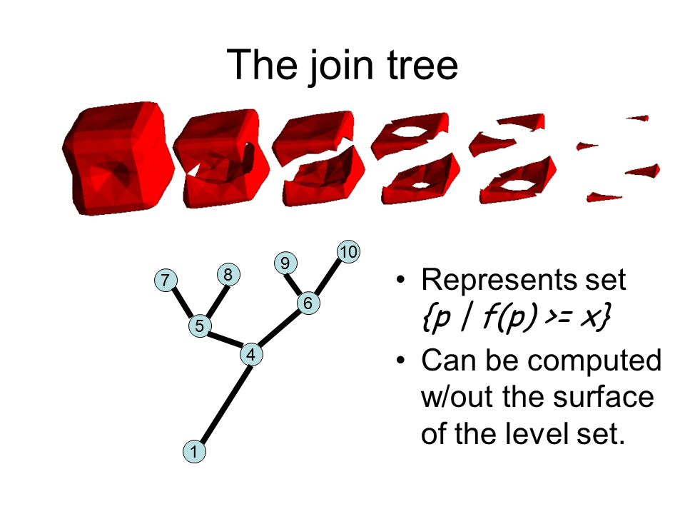
55. The join tree Represents set {p | f(p) >= x} Can be computed w/out the surface of the level set. 7 8 9 10 5 6 4 1

56. Join tree construction Sort data by  value Maintain union/find for comp. of {p | f(p) >= x} 7 8 9 10 5 6 4

57. Union/Find Data structure for integers 1..n supporting: –Initialize() each integer starts in its own group for i = 1..n, g(i) = i; –Union(i,j) union groups of i and j g(Find(i)) = Find(j); –Find(i) return name of group containing i group = i; while group != g(group), group = g(group); // find group while i != group, {nx = g(i), g(i) = group, i = nx} // compress path Does n union/finds in O(n a(n)) steps [T72]

58. Join tree construction Sort data by  value Maintain union/find for comp. of {p | f(p) >= x} O(n+ t·α ( t ) ) after sort 7 8 9 10 5 6 4 1

59. The split tree 10 3 1 2 Represents the set {p | f(p) <= x} Reverse join tree computation

60. Merge join and split trees 10 3 1 2 7 8 9 5 6 4 1 7 8 9 5 6 4 3 1 2

61. Merge join and split trees Algorithm

62. 1. Add nodes from other tree Nodes have correct up degree in join & down degree in the split tree. 7 8 9 10 5 6 4 1 7 8 9 5 6 4 3 1 2 3 2

63. 2. Identify leaves A leaf in one tree, with up/down degree < 1 in other tree 7 8 9 10 5 6 4 1 7 8 9 5 6 4 3 1 2 3 2

64. 3. Add to contour tree A leaf in one tree, with up/down degree < 1 in other tree 7 8 9 10 5 6 4 1 7 8 9 5 6 4 3 1 3 3 2

65. 3. Add to contour tree 7 8 9 10 5 6 4 1 7 8 9 5 6 4 3 1 3 3 2

66. 3. Add to contour tree 7 8 9 10 5 6 4 7 8 9 5 6 4 3 1 3 3 2

67. 3. Add to contour tree Note that 4 is not a leaf 7 8 9 10 5 6 4 7 8 9 5 6 4 1 3 2 4

68. 3. Add to contour tree The merge time is proportional to the tree size; much smaller than the data 8 9 10 5 6 4 8 9 5 6 4 1 3 2 4 7 5

69. 4. Ends with Contour tree 7 8 9 10 5 6 4 3 1 2

70. Advantages Doesn’t need the surface structure to build the contour tree. The merge becomes simple, and works on a subset of the points The tree structure can advise where to choose the threshold value Can cut diff. branches at diff. values.

71. Flexible contouring Threshold diff. areas at diff. values

72. Flexible contouring Threshold diff. areas at diff. Values Guided by the Contour Tree 7 8 9 10 5 6 4 3 1 2

73. Properties Display of Level Sets Topology (Structural Information) –Merge, Split, Create, Disappear, Genus Change (Betti number change) Minimal Seed Set Generation Contour Segmentation –A point on any edge of CT corresponds to one contour component

74. Contour Tree Drawing and UI

75. Hybrid Parallel Contour Extraction Different from isocontour extraction Divide contour extraction process into –Propagation Iterative algorithm -> hard to optimize using GPU multi-threaded algorithm executed in multi-core CPU –Triangulation CUDA implementation executed in many-core GPU 75

76. Hybrid Parallel Contour Extraction

77. Results

78. Interactive Interface with Quantitative Information Geometric Property as saliency level –Gradient(color) + Area (thickness) 78

79. Segmentation of Regions of Interest Mass Segmentation from Mammograms Minimum Nesting Depth (MND) –Measured for each node of contour tree –MND = min (depth from current node to terminal node of every subtree) –High MND contour represents the boundaries of distinctive regions with abrupt intensity changes retaining the same topology –Successfully applied to mass detection from 400 mammograms in USF database. 79

80. Salient Isosurface Extraction How to select isovalue? Contour Spectrum –[ Bajaj et al. VIS97 ] –shows quantitative properties (area, volume, gradient) for all isovalues –allows semi-automatic isovalue selection

81. Isovalue Selection The contour spectrum allows the development of an adaptive ability to separate interesting isovalues from the others.

82. Contour Spectrum (CT scan of an engine) The contour spectrum allows the development of an adaptive ability to separate interesting isovalues from the others.

83. Salient Contour Extraction Using Contour Tee 83

84. Motivation Infinitely many isocontours defined in an image An isocontour may have many contours Contour –Connected component of an isocontour –Often represents an independent structure 84 Ex) mammogram (X-ray exam of female breast)

85. Motivation Salient Contour Extraction –Useful for segmentation, analysis and visualization of regions of interest –Can be applied to CAD(Computer Aided Diagnosis) for detecting suspicious regions 85 mass (tumor) dense tissue breast boundarypectoral muscle

86. 3D Examples 86

87. Past Contour Tree Approach Contour Tree –Represents topological changes of contours according to isovalue change. –Property structure (topology) of level sets contour extraction seed set generation for fast extraction 87

88. Our Approach Interactive Contour Tree Interface –Performance Improvement of Extraction Process –Utilizing Quantitative Information Development of Saliency Metric –MND(Minimum Nesting Depth) –Apply to medical images 88

89. Hybrid Parallel Contour Extraction Different from isocontour extraction Divide contour extraction process into –Propagation Iterative algorithm -> hard to optimize using GPU multi-threaded algorithm executed in multi-core CPU –Triangulation CUDA implementation executed in many-core GPU 89

90. Interactive Interface with Quantitative Information Geometric Property as saliency level –Gradient(color) + Area (thickness) 90

91. Saliency Metric Minimum Nesting Depth (MND) –Measured for each node of contour tree –MND = min (depth from current node to terminal node of every subtree) –High MND contour represents the boundaries of distinctive regions with abrupt intensity changes retaining the same topology –Successfully applied to mass detection from 400 mammograms in USF database. 91