2. Announcements Phrases assignment out today: – Unsupervised learning – Google n-grams data – Non-trivial pipeline – Make sure you allocate time to actually run the program Hadoop assignment (out next week): – Streaming Hadoop first, then “real” Hadoop Streaming Hadoop a “checkpoint” not an assignment – Time to master Amazon cloud and Hadoop mechanics

3. Review/outline Streaming learning algorithms – Naïve Bayes – Rocchio’s algorithm Similarities & differences – Probabilistic vs vector space models – Computationally: linear classifiers (inner product x and v (y)) constant number of passes over data very simple with word counts in memory pretty simple for large vocabularies trivially parallelized adding operations Alternative: – Adding up contributions for every example vs conservatively updating a linear classifier – On-line learning model: mistake-bounds

4. Review/outline Streaming learning algorithms … and beyond – Naïve Bayes – Rocchio’s algorithm Similarities & differences – Probabilistic vs vector space models – Computationally similar – Parallelizing Naïve Bayes and Rocchio Alternative: – Adding up contributions for every example vs conservatively updating a linear classifier – On-line learning model: mistake-bounds some theory a mistake bound for perceptron – Parallelizing the perceptron

6. Parallel Rocchio - pass 1 Documents/labels Documents/labels – 1 Documents/labels – 2 Documents/labels – 3 DFs -1 DFs - 2 DFs -3 DFs Split into documents subsets Sort and add counts Compute DFs “extra” work in parallel version

7. Parallel Rocchio - pass 2 Documents/labels Documents/labels – 1 Documents/labels – 2 Documents/labels – 3 v-1 v-2 v-3 DFs Split into documents subsets Sort and add vectors Compute partial v ( y)’s v ( y )’s extra work in parallel version

8. Limitations of Naïve Bayes/Rocchio Naïve Bayes: one pass Rocchio: two passes – if vocabulary fits in memory Both method are algorithmically similar – count and combine Thought thought thought thought thought thought thought thought thought thought experiment: what if we duplicated some features in our dataset many times times times times times times times times times times? – e.g., Repeat all words that start with “t” “t” “t” “t” “t” “t” “t” “t” “t” “t” ten ten ten ten ten ten ten ten ten ten times times times times times times times times times times. – Result: those features will be over-weighted in classifier by a factor of 10 This isn’t silly – often there are features that are “noisy” duplicates, or important phrases of different length

9. One simple way to look for interactions Naïve Bayes sparse vector of TF values for each word in the document…pl us a “bias” term for f(y) dense vector of g(x,y) scores for each word in the vocabulary.. plus f(y) to match bias term

10. One simple way to look for interactions Naïve Bayes – two class version dense vector of g(x,y) scores for each word in the vocabulary Scan thru data: whenever we see x with y we increase g(x,y)-g(x,~y) whenever we see x with ~ y we decrease g(x,y)-g(x,~y) Scan thru data: whenever we see x with y we increase g(x,y)-g(x,~y) whenever we see x with ~ y we decrease g(x,y)-g(x,~y) To detect interactions: increase/decrease g(x,y)-g(x,~y) only if we need to (for that example) otherwise, leave it unchanged To detect interactions: increase/decrease g(x,y)-g(x,~y) only if we need to (for that example) otherwise, leave it unchanged

11. A “Conservative” Streaming Algorithm is Sensitive to Duplicated Features B instance x i Compute: y i = v k. x i ^ +1,-1: label y i If mistake: v k+1 = v k + correction Train Data To detect interactions: increase/decrease v k only if we need to (for that example) otherwise, leave it unchanged (“conservative”) We can be sensitive to duplication by coupling updates to feature weights with classifier performance (and hence with other updates ) To detect interactions: increase/decrease v k only if we need to (for that example) otherwise, leave it unchanged (“conservative”) We can be sensitive to duplication by coupling updates to feature weights with classifier performance (and hence with other updates )

12. Parallel Rocchio Documents/labels Documents/labels – 1 Documents/labels – 2 Documents/labels – 3 v-1 v-2 v-3 DFs Split into documents subsets Sort and add vectors Compute partial v ( y)’s v ( y )’s

13. Parallel Conservative Learning Documents/labels Documents/labels – 1 Documents/labels – 2 Documents/labels – 3 v-1 v-2 v-3 Classifier Split into documents subsets Compute partial v ( y)’s v ( y )’s Key Point: We need shared write access to the classifier – not just read access. So we only need to not copy the information but synchronize it. Question: How much extra communication is there? Like DFs or event counts, size is O(|V|)

14. Parallel Conservative Learning Documents/labels Documents/labels – 1 Documents/labels – 2 Documents/labels – 3 v-1 v-2 v-3 Classifier Split into documents subsets Compute partial v ( y)’s v ( y )’s Key Point: We need shared write access to the classifier – not just read access. So we only need to not copy the information but synchronize it. Question: How much extra communication is there? Answer: Depends on how the learner behaves… …how many weights get updated with each example … (in Naïve Bayes and Rocchio, only weights for features with non-zero weight in x are updated when scanning x ) …how often it needs to update weight … (how many mistakes it makes) Like DFs or event counts, size is O(|V|)

15. Review/outline Streaming learning algorithms … and beyond – Naïve Bayes – Rocchio’s algorithm Similarities & differences – Probabilistic vs vector space models – Computationally similar – Parallelizing Naïve Bayes and Rocchio easier than parallelizing a conservative algorithm? Alternative: – Adding up contributions for every example vs conservatively updating a linear classifier – On-line learning model: mistake-bounds some theory a mistake bound for perceptron – Parallelizing the perceptron

16. A “Conservative” Streaming Algorithm B instance x i Compute: y i = v k. x i ^ +1,-1: label y i If mistake: v k+1 = v k + correction Train Data

17. Theory: the prediction game Player A: – picks a “target concept” c for now - from a finite set of possibilities C (e.g., all decision trees of size m) – for t=1,…., Player A picks x =(x 1,…,x n ) and sends it to B – For now, from a finite set of possibilities (e.g., all binary vectors of length n) B predicts a label, ŷ, and sends it to A A sends B the true label y =c( x ) we record if B made a mistake or not – We care about the worst case number of mistakes B will make over all possible concept & training sequences of any length The “Mistake bound” for B, M B (C), is this bound

18. Some possible algorithms for B The “optimal algorithm” – Build a min-max game tree for the prediction game and use perfect play not practical – just possible C 0001 1011 ŷ(01)=0ŷ(01)=1 y=0y=1 {c in C:c(01)=1} {c in C: c(01)=0}

19. Some possible algorithms for B The “Halving algorithm” – Remember all the previous examples – To predict, cycle through all c in the “version space” of consistent concepts in c, and record which predict 1 and which predict 0 – Predict according to the majority vote Analysis: – With every mistake, the size of the version space is decreased in size by at least half – So M halving (C) <= log 2 (|C|) not practical – just possible

20. More results A set s is “ shattered ” by C if for any subset s ’ of s, there is a c in C that contains all the instances in s’ and none of the instances in s-s’. The “ VC dimension ” of C is | s |, where s is the largest set shattered by C. VCdim is closely related to pac-learnability of concepts in C.

21. More results A set s is “ shattered ” by C if for any subset s ’ of s, there is a c in C that contains all the instances in s’ and none of the instances in s-s’. The “ VC dimension ” of C is | s |, where s is the largest set shattered by C.

22. More results A set s is “ shattered ” by C if for any subset s ’ of s, there is a c in C that contains all the instances in s’ and none of the instances in s-s’. The “ VC dimension ” of C is | s |, where s is the largest set shattered by C. C 0001 1011 ŷ(01)=0ŷ(01)=1 y=0y=1 {c in C:c(01)=1} {c in C: c(01)=0} Theorem: M opt (C)>=VC(C) Proof: game tree has depth >= VC(C)

23. More results A set s is “ shattered ” by C if for any subset s ’ of s, there is a c in C that contains all the instances in s’ and none of the instances in s-s’. The “ VC dimension ” of C is | s |, where s is the largest set shattered by C. C 0001 1011 ŷ(01)=0ŷ(01)=1 y=0y=1 {c in C:c(01)=1} {c in C: c(01)=0} Corollary: for finite C VC(C) <= M opt (C) <= log2(|C|) Proof: M opt (C) <= M halving (C) <=log2(|C|)

24. More results A set s is “ shattered ” by C if for any subset s ’ of s, there is a c in C that contains all the instances in s’ and none of the instances in s-s’. The “ VC dimension ” of C is | s |, where s is the largest set shattered by C. Theorem: it can be that M opt (C) >> VC(C) Proof: C = set of one- dimensional threshold functions. + - ?

25. The prediction game Are there practical algorithms where we can compute the mistake bound?

26. The perceptron game A B instance x i Compute: y i = sign(v k. x i ) ^ y i ^ If mistake: v k+1 = v k + y i x i x is a vector y is -1 or +1

27. u -u 2γ2γ u -u-u 2γ2γ +x1+x1 v1v1 (1) A target u (2) The guess v 1 after one positive example. u -u 2γ2γ u -u-u 2γ2γ v1v1 +x2+x2 v2v2 +x1+x1 v1v1 -x2-x2 v2v2 (3a) The guess v 2 after the two positive examples: v 2 =v 1 +x 2 (3b) The guess v 2 after the one positive and one negative example: v 2 =v 1 -x 2 If mistake: v k+1 = v k + y i x i

28. u -u 2γ2γ u -u-u 2γ2γ v1v1 +x2+x2 v2v2 +x1+x1 v1v1 -x2-x2 v2v2 (3a) The guess v 2 after the two positive examples: v 2 =v 1 +x 2 (3b) The guess v 2 after the one positive and one negative example: v 2 =v 1 -x 2 >γ>γ If mistake: v k+1 = v k + y i x i

29. u -u 2γ2γ u -u-u 2γ2γ v1v1 +x2+x2 v2v2 +x1+x1 v1v1 -x2-x2 v2v2 (3a) The guess v 2 after the two positive examples: v 2 =v 1 +x 2 (3b) The guess v 2 after the one positive and one negative example: v 2 =v 1 -x 2 If mistake: y i x i v k < 0

31. 2 2 2 2 2 Notation fix to be consistent with next paper

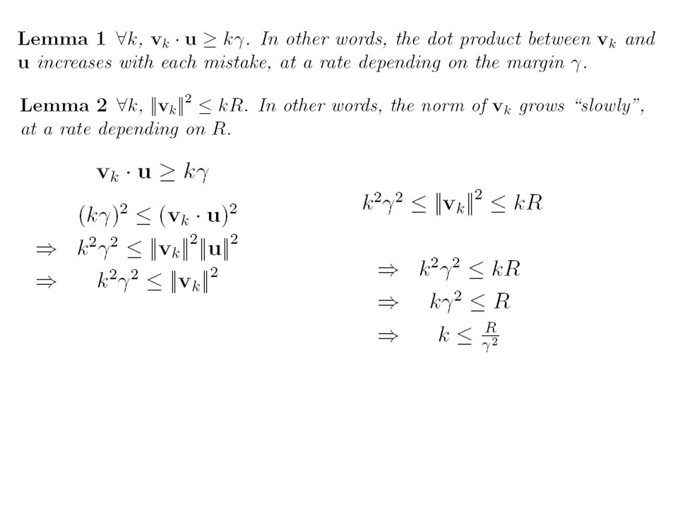
32. Summary We have shown that –If : exists a u with unit norm that has margin γ on examples in the seq (x 1,y 1 ),(x 2,y 2 ),…. –Then : the perceptron algorithm makes = ||x i ||) –Independent of dimension of the data or classifier (!) –This doesn’t follow from M(C)<=VCDim(C) We don’t know if this algorithm could be better –There are many variants that rely on similar analysis (ROMMA, Passive-Aggressive, MIRA, …) We don’t know what happens if the data’s not separable –Unless I explain the “Δ trick” to you We don’t know what classifier to use “after” training

33. The Δ Trick Replace x i with x’ i so X becomes [X | I Δ] Replace R 2 in our bounds with R 2 + Δ 2 Let d i = max(0, γ - y i x i u) Let u’ = (u 1,…,u n, y 1 d 1 /Δ, … y m d m /Δ) * 1/Z –So Z=sqrt(1 + D 2 / Δ 2 ), for D=sqrt(d 1 2 +…+d m 2 ) Mistake bound is (R 2 + Δ 2 )Z 2 / γ 2 Let Δ = sqrt(RD)  k <= ((R + D)/ γ) 2

34. Summary We have shown that –If : exists a u with unit norm that has margin γ on examples in the seq (x 1,y 1 ),(x 2,y 2 ),…. –Then : the perceptron algorithm makes = ||x i ||) –Independent of dimension of the data or classifier (!) We don’t know what happens if the data’s not separable –Unless I explain the “Δ trick” to you We don’t know what classifier to use “after” training

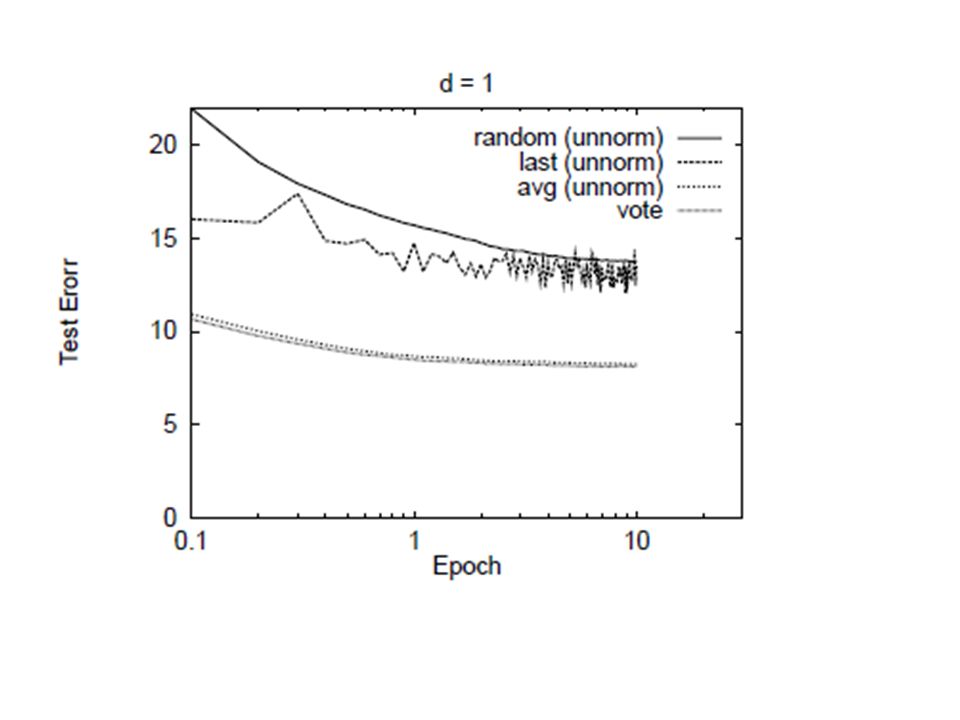
35. On-line to batch learning 1.Pick a v k at random according to m k /m, the fraction of examples it was used for. 2.Predict using the v k you just picked. 3.(Actually, use some sort of deterministic approximation to this).

37. Complexity of perceptron learning Algorithm: v=0 for each example x, y: – if sign( v.x) != y v = v + y x init hashtable for x i !=0, v i += y x i O(n) O(| x |)=O(|d|)

38. Complexity of averaged perceptron Algorithm: vk=0 va = 0 for each example x, y: – if sign( vk.x) != y va = va + nk vk vk = vk + y x nk = 1 – else nk++ init hashtables for vk i !=0, va i += vk i for x i !=0, v i += y x i O(n) O(n|V|) O(| x |)=O(|d|) O(|V|) So: averaged perceptron is better from point of view of accuracy (stability, …) but much more expensive computationally.

39. Complexity of averaged perceptron Algorithm: vk=0 va = 0 for each example x, y: – if sign( vk.x) != y va = va + nk vk vk = vk + y x nk = 1 – else nk++ init hashtables for vk i !=0, va i += vk i for x i !=0, v i += y x i O(n) O(n|V|) O(| x |)=O(|d|) O(|V|) The non-averaged perceptron is also hard to parallelize…

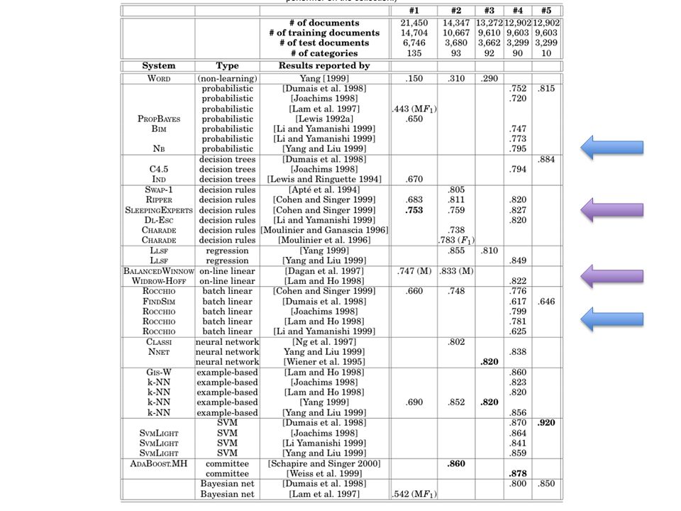
40. A hidden agenda Part of machine learning is good grasp of theory Part of ML is a good grasp of what hacks tend to work These are not always the same – Especially in big-data situations Catalog of useful tricks so far – Brute-force estimation of a joint distribution – Naive Bayes – Stream-and-sort, request-and-answer patterns – BLRT and KL-divergence (and when to use them) – TF-IDF weighting – especially IDF it’s often useful even when we don’t understand why – Perceptron often leads to fast, competitive, easy-to-implement methods averaging helps what about parallel perceptrons?

41. Parallel Conservative Learning Documents/labels Documents/labels – 1 Documents/labels – 2 Documents/labels – 3 v-1 v-2 v-3 Classifier Split into documents subsets Compute partial v ( y)’s v ( y )’s vk/va

42. Parallelizing perceptrons Instances/labels Instances/labels – 1 Instances/labels – 2 Instances/labels – 3 vk/va -1 vk/va- 2 vk/va-3 vk Split into example subsets Combine somehow? Compute vk’s on subsets

43. NAACL 2010

44. Aside: this paper is on structured perceptrons …but everything they say formally applies to the standard perceptron as well Briefly: a structured perceptron uses a weight vector to rank possible structured predictions y’ using features f ( x,y’ ) Instead of incrementing weight vector by y x, the weight vector is incremented by f(x,y) - f ( x,y’)

45. Parallel Perceptrons Simplest idea: – Split data into S “shards” – Train a perceptron on each shard independently weight vectors are w (1), w (2), … – Produce some weighted average of the w (i) ‘s as the final result

46. Parallelizing perceptrons Instances/labels Instances/labels – 1 Instances/labels – 2 Instances/labels – 3 vk -1 vk- 2 vk-3 vk Split into example subsets Combine by some sort of weighted averaging Compute vk’s on subsets

47. Parallel Perceptrons Simplest idea: – Split data into S “shards” – Train a perceptron on each shard independently weight vectors are w (1), w (2), … – Produce some weighted average of the w (i) ‘s as the final result Theorem: this doesn’t always work. Proof: by constructing an example where you can converge on every shard, and still have the averaged vector not separate the full training set – no matter how you average the components.

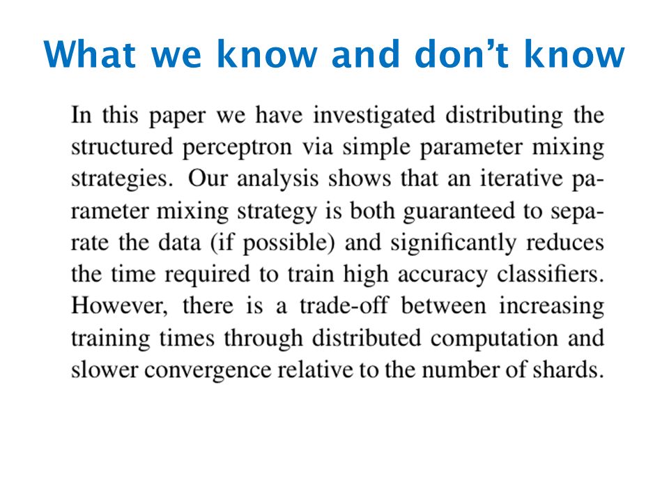
48. Parallel Perceptrons – take 2 Idea: do the simplest possible thing iteratively. Split the data into shards Let w = 0 For n=1,… Train a perceptron on each shard with one pass starting with w Average the weight vectors (somehow) and let w be that average Extra communication cost: redistributing the weight vectors done less frequently than if fully synchronized, more frequently than if fully parallelized

49. Parallelizing perceptrons – take 2 Instances/labels Instances/labels – 1 Instances/labels – 2 Instances/labels – 3 w -1 w- 2 w-3 w w Split into example subsets Combine by some sort of weighted averaging Compute local vk’s w (previous)

50. A theorem Corollary: if we weight the vectors uniformly, then the number of mistakes is still bounded. I.e., this is “enough communication” to guarantee convergence.

51. What we know and don’t know uniform mixing… μ =1/S could we lose our speedup-from- parallelizing to slower convergence?

52. Results on NER

53. Results on parsing

54. The theorem…

57. IH1 inductive case: γ

58. Review/outline Streaming learning algorithms … and beyond – Naïve Bayes – Rocchio’s algorithm Similarities & differences – Probabilistic vs vector space models – Computationally similar – Parallelizing Naïve Bayes and Rocchio Alternative: – Adding up contributions for every example vs conservatively updating a linear classifier – On-line learning model: mistake-bounds some theory a mistake bound for perceptron – Parallelizing the perceptron

59. What we know and don’t know uniform mixing… could we lose our speedup-from- parallelizing to slower convergence?

60. What we know and don’t know

63. Review/outline Streaming learning algorithms … and beyond – Naïve Bayes – Rocchio’s algorithm Similarities & differences – Probabilistic vs vector space models – Computationally similar – Parallelizing Naïve Bayes and Rocchio Alternative: – Adding up contributions for every example vs conservatively updating a linear classifier – On-line learning model: mistake-bounds some theory a mistake bound for perceptron – Parallelizing the perceptron

64. Where we are… Summary of course so far: – Math tools: complexity, probability, on-line learning – Algorithms: Naïve Bayes, Rocchio, Perceptron, Phrase- finding as BLRT/pointwise KL comparisons, … – Design patterns: stream and sort, messages How to write scanning algorithms that scale linearly on large data (memory does not depend on input size) – Beyond scanning: parallel algorithms for ML – Formal issues involved in parallelizing Naïve Bayes, Rocchio, … easy? Conservative on-line methods (e.g., perceptron) … hard? Next: practical issues in parallelizing – details on Hadoop