1. Week 15 – Wednesday

2.  What did we talk about last time?  Review up to Exam 1

4. Graphic Violence

6. public class ArrayList { private String[] array = new String[10]; private int size = 0; … } Complete the following a method to insert a value in an arbitrary index in the list. You may have to resize the list if it doesn't have enough space. public void insert(String value, int index)

7. public class Tree { public static class Node { public String key; public Node left; public Node right; } private Node root = null; … } public class List { public static class Node { public String value; public Node next; } private Node head = null; … }

8.  Write a method in the List class that will remove every other node (the even numbered nodes) from a linked list public void removeAlternateNodes()

12.  Base case  Tells recursion when to stop  Can have multiple base cases  Have to have at least one or the recursion will never end  Recursive case  Tells recursion how to proceed one more step  Necessary to make recursion able to progress  Multiple recursive cases are possible

13.  Factorial: int factorial( int n ) { if( n == 1 ) return 1; else return n * factorial( n – 1); }

14.  We can define the running time of a function as a relation of the form: T(1) = c T(n) = a T(f(n)) + g(n) Example using factorial: T(1) = 1 T(n) = T(n - 1) + 1

16.  Given an N x N chess board, where N ≥ 4 it is possible to place N queens on the board so that none of them are able to attack each other in a given move  Write a method that, given a value of N, will return the total number of ways that the N queens can be placed

17.  A symbol table goes by many names:  Map  Lookup table  Dictionary  The idea is a table that has a two columns, a key and a value  You can store, lookup, and change the value based on the key

18.  We can define a symbol table ADT with a few essential operations:  put(Key key, Value value) ▪ Put the key-value pair into the table  get(Key key): ▪ Retrieve the value associated with key  delete(Key key) ▪ Remove the value associated with key  contains(Key key) ▪ See if the table contains a key  isEmpty()  size()  It's also useful to be able to iterate over all keys

20.  A tree is a data structure built out of nodes with children  A general tree node can have any non- negative number of children  Every child has exactly one parent node  There are no loops in a tree  A tree expressions a hierarchy or a similar relationship

21.  The root is the top of the tree, the node which has no parents  A leaf of a tree is a node that has no children  An inner node is a node that does have children  An edge or a link connects a node to its children  The depth of a node is the length of the path from a node to its root  The height of the tree is the greatest depth of any node  A subtree is a node in a tree and all of its children  Level: the set of all nodes at a given depth from the root

22. 1 1 2 2 3 3 4 4 5 5 6 6 7 7 Root Inner Nodes Leaves

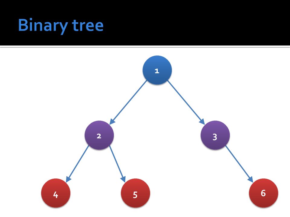
23.  A binary tree is a tree such that each node has two or fewer children  The two children of a node are generally called the left child and the right child, respectively

24. 1 1 2 2 3 3 4 4 5 5 6 6

25.  Full binary tree: every node other than the leaves has two children  Perfect binary tree: a full binary tree where all leaves are at the same depth  Complete binary tree: every level, except possibly the last, is completely filled, with all nodes to the left  Balanced binary tree: the depths of all the leaves differ by at most 1

26.  A binary search tree is binary tree with three properties: 1. The left subtree of the root only contains nodes with keys less than the root’s key 2. The right subtree of the root only contains nodes with keys greater than the root’s key 3. Both the left and the right subtrees are also binary search trees

27.  Keeping data organized  Easy to produce a sorted order in O(n) time  Find, add, and delete are all O(log n) time

28. public class Tree { private static class Node { public int key; public String value; public Node left; public Node right; } private Node root = null; … }

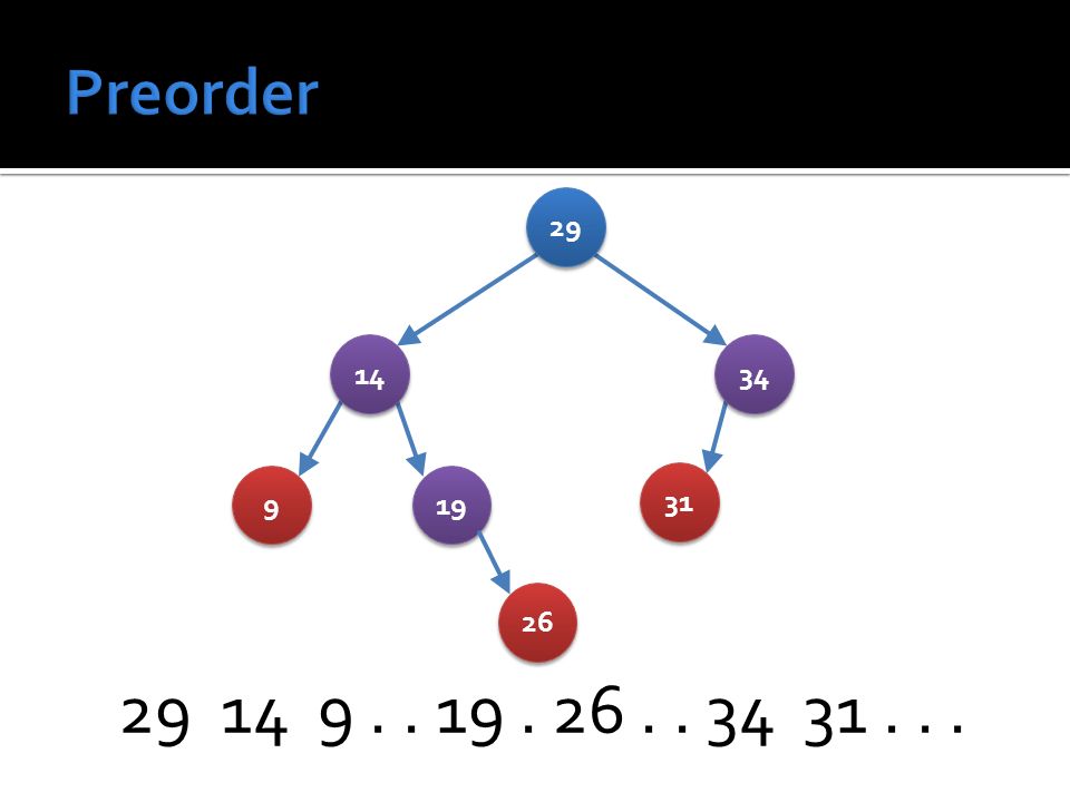
29. 29 14 9.. 19. 26.. 34 31... 29 14 34 9 9 19 31 26

30. .. 9... 26 19 14.. 31. 34 29 29 14 34 9 9 19 31 26

31. . 9. 14. 19. 26. 29. 31. 34. 29 14 34 9 9 19 31 26

32. 29 14 34 9 19 31.... 26.... 29 14 34 9 9 19 31 26

33.  For depth first traversals, we used a stack  What are we going to use for a BFS?  A queue!  Algorithm: 1. Put the root of the tree in the queue 2. As long as the queue is not empty: a)Dequeue the first element and process it b)Enqueue all of its children

34.  We can have a balanced tree by:  Doing red-black (or AVL) inserts  Balancing a tree by construction (sort, then add)  DSW algorithm: completely unbalance then rebalance

35.  A 2-3 search tree is a data structure that maintains balance  It is actually a ternary tree, not a binary tree  A 2-3 tree is one of the following three things:  An empty tree (null)  A 2-node (like a BST node) with a single key, smaller data on its left and larger values on its right  A 3-node with two keys and three links, all key values smaller than the first key on the left, between the two keys in the middle, and larger than the second key on the right

36.  The key thing that keeps a 2-3 search tree balanced is that all leaves are on the same level  Only leaves have null links  Thus, the maximum depth is somewhere between the log 3 n (the best case, where all nodes are 3-nodes) and log 2 n (the worst case, where all nodes are 2-nodes)

37.  We build from the bottom up  Except for an empty tree, we never put a new node in a null link  Instead, you can add a new key to a 2-node, turning it into a 3-node  Adding a new key to a 3-node forces it to break into two 2-nodes

39.  We can do an insertion with a red-black tree using a series of rotations and recolors  We do a regular BST insert  Then, we work back up the tree as the recursion unwinds  If the right child is red and the left is black, we rotate the current node left  If the left child is red and the left child of the left child is red, we rotate the current node right  If both children are red, we recolor them black and the current node red  You have to do all these checks, in order!  Multiple rotations can happen  It doesn't make sense to have a red root, so we always color the root black after the insert

40. We perform a left rotation when the right child is red Y Y X X B B A A C C Current Y Y X X B B A A C C

41. We perform a right rotation when the left child is red and its left child is red Z Z Y Y B B A A D D Current X X C C Z Z Y Y B B A A D D X X C C

42. We recolor both children and the current node when both children are red Y Y X X B B A A D D Current Z Z C C Y Y X X B B A A D D Z Z C C

43.  Learn how to do 2-3 tree insertions really well  Then, learn how you can map a 2-3 tree onto a red-back tree  It's much easier to make a 2-3 tree and then figure out the corresponding red-black tree than it is to build a red-black tree from scratch

45.  We make a huge array, so big that we’ll have more spaces in the array than we expect data values  We use a hashing function that maps items to indexes in the array  Using the hashing function, we know where to put each item but also where to look for a particular item

46.  We are using a hash table for a space/time tradeoff  Lots of space means we can get down to O(1)  How much space do we need?  When the table gets too full, we may need to rehash everything  How do we pick a good hashing function?  What happens if two values collide (map to the same location)

47.  With open addressing, we look for some empty spot in the hash table to put the item  There are a few common strategies  Linear probing  Quadratic probing  Double hashing  Alternatively, we can use chaining

50.  Finish student questions  Review everything after Exam 2  Graphs  Shortest paths  Minimum spanning trees  Eulerian tours and paths  Hamiltonian tours  Matching  Sorting  Heaps  Tries  Review Chapters 4, 2, and sections 5.1 and 5.2

51.  Finish Project 4  Due Friday  Study for final exam  2:30 - 5:30pm, Monday, 12/07/2015