1. NASA, JPL,January 2011

2.  CLIME INRIA Paris  Météo France  Institut de Mathématiques, Université de Toulouse  LEGI, Grenoble  MOISE INRIA Grenoble and Université de Grenoble

3.  Observing the Earth with satellites.  Data Assimilation.  Images.  Plugging images into numerical models.  Variational approach.  Pseudo-Observations methods.  Direct Assimilation of Images Sequences.  Operational Applications  Perspectives

4.  Numerical models are not sufficient to carry out a prediction.  Numerical models are based on non linear PDE’s and after a spatial discretisation a system of first order ODE’s of huge dimensionnality (at the present time around one billions of equations for operational models.  Prediction is obtained by an integration of the model starting from an initial condition.  The process necessary for obtaining an initial condition from data is named Data Assimilation

5.  Basically it’s a ill-posed problem : about 10 millions of daily data to retrieve 1 billions of unknowns  Interpolation methods are not sufficient to obtain consistant fields (with respect to fluid dynamics)  Variational Methods are based on Optimal Control Methods and are presently used by the main meteorological centers  Kalman filter approach is used in mainly in a research context

6.  Images provided by the observation of the earth quantity a large amount of information  This information is used in a qualitative way rather than in a quantitative one.  How to couple this source of information with mathematical models in order to improve prediction?

7. ICTMA 13 NOAA AMSUA/B HIRS, AQUA AIRS DMSP SSM/I SCATTEROMETERS GEOS TERRA / AQUA MODIS OZONE 27 satellite data sources used in 4D-Var

8. ICTMA 13

13.  Images are defined by pixels  For black and white image each pixel is associated with a grey level (0<gl<1). For Meteosat 256 grey levels  For color images each pixel is associated to 3 numbers.  Each image (Meteosat) has around 25 millions of pixels.  A full sequence of images is a very large data set and cannot be directly used in an operational context

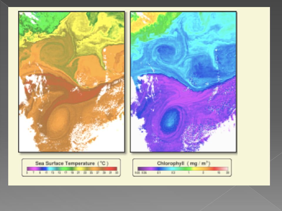
14.  The basic variables of meteorological models are : wind, temperature, humidity, atmospheric pressure only humidity can be seen on some satellites.  For oceanic models : stream, temperature, salinity, surface elevation. Only salinity and temperature give images.  For the atmosphere the images represent the integral of the radiative properties of the atmosphere.  For the ocean the images represent the surface values of the radiative properties of the ocean  Information in images is borne by the discontinuities in the images (e.g. fronts)  Images of the ocean can be occulted by clouds.

19.  Based on laws of conservation (mass, energy)  Nonlinear PDE’s linking the state variables of the model  To use images it is necessary to introduce the evolution of the quantities dispalyed by images: › Humidity (for meteorological models) › Salinity (for oceanic models) › Conservation of a (supposed to be) passive tracer (e.g. phyloplakton in oceanic models) › Conservation of luminance › In any case a complexification of the models if images are taken into account.

23.  Pseudo Observations Methods. › From images velocities are extracted, then used as regular observations.  Direct Assimilation of Images. › An extra term is added in the cost function evaluating the discrepancy between the pseudo-images issued from the numerical model and the oberved image, then the usual tools of VDA are used

25.  The temporal coherency of a sequence of image is obtained by a law of conservation of brightness   If the gradient of brightness and the velocity are orthogonal then no information is added (if an image is uniform then it can’t provide information on velocity)  How to isolate structures such that this equation is representative of the flow?

26.  Recovering U from I is a ill posed problem  Introducing a problem of optimization

28.  The minimization of the cost function is performed in nested subspaces of admissible deplacements fields at scale q. It contains piecewise affine vector fields with respect to each space variables on a square of size qxq pixels.  In practice with 2 successive time steps

41.  Model Image methods do no take into account the physical properties of the fields issued from fluid mechanics.  The retrieved field can be coherent but with few physical sense.  The idea is to add to the optimization problem a physical constraint issued from the equation governing the fields.

59.  FSLE is a Lagrangian tool to characterize coherent structures in time-dependant flows.  Widely used in oceanography to link ocean tracer distribution with mesoscale geostrophic currents in order to study stirring and mixing processes.  FTLE are not directly observed but extracted from the ocean tracer images

62.  For a 2D decaying turbulent flow, the orientation of the gradient of the concentration of a passive tracer converges to backward FLTV orientation

67.  Structure are extracted by applying a threshold of the gradient of concentration.  Same operation is carried out on the results of the numerical model.  The comparison between these structures is done on the associated FTLE

68.  Evolution of dry intrusion in cyclogenesis  Follow-up of convective cells in radar meteorology : short term prediction of severe storms

69.  Images have a strong predictive potential  Images can be plugged in numerical models  Some new developments are underway for the study and parametrization of turbulence  Other developments e.g. in heart modelling and other scientific fields