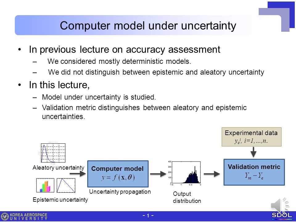
2. - 1 - Computer model under uncertainty In previous lecture on accuracy assessment –We considered mostly deterministic models. – We did not distinguish between epistemic and aleatory uncertainty In this lecture, –Model under uncertainty is studied. –Validation metric distinguishes between aleatory and epistemic uncertainties. Aleatory uncertainty Computer model Uncertainty propagation Output distribution Validation metric Experimental data y e i, i=1,…,n. Epistemic uncertainty

3. - 2 - Nonlinearity effect with aleatory uncertainty Example 1 –Computer model: –Deterministic solution: at x = 3.5, y = 6.452 –Stochastic solution under aleatory uncertainty Aleatory uncertainty: inherent randomness, irreducible. Ex: material variability, sensor noise, uncontrolled environments Input uncertainty: x ~ N(  X  2 ), where mean  X = 3.5, stdev  = 1.2. Output is obtained by crude Monte-Carlo simulation with N=1e5. Matlab code in notes for mean standard deviation and CDF Result [mean, std]=[5.967, 1.125] Run again obtained [5.968, 1.121] O’Hagan, "Bayesian analysis of computer code outputs: a tutorial." RESS 91.10 (2006): 1290-1300

4. - 3 - Epistemic sampling uncertainty Example 1 –Stochastic solution under epistemic uncertainty (case 1:limited data) Epistemic uncertainty: lack of knowledge, reducible. Ex: limited number of data, poor knowledge about boundary conditions –Input x is given with only a few data: n=5, mx=3.5, stdev=1.2. –For simplicity stdev assumed known. Posterior distribution of unknown mean –Double loop process Samples of mean of x are drawn from its posterior distribution with N1=50.(left figure) For each mean Monte-Carlo simulation with N=1e5 generates CDF (right figure) Matlab codes given in notes page O’Hagan, "Bayesian analysis of computer code outputs: a tutorial." RESS

5. - 4 - Epistemic uncertainty about a constant Example 1 –Computer model: –Stochastic solution under epistemic uncertainty (case 2:vague knowledge) –Parameter u is given with interval: u ~ (1.5,2.5) was 2 before –Double loop process 50 samples of u are drawn from its distribution. CDFs are obtained by Monte-Carlo simulation with N=1e5 at each u sample. We get 50 CDF’s, representing vague knowledge. Code is in the note page. O’Hagan, "Bayesian analysis of computer code outputs: a tutorial." RESS

6. Vote Is this procedure of separating epistemic and aleatory uncertainty more sensible than lumping them together? Lumping together means taking the 50 times 100,000 samples and generating a single CDF. A key question is how do you impart the uncertainty in your probability estimates.

7. - 6 - Example 2: Heat transfer through a solid –Problem SRQ is the heat flux q w through the left end of a solid metal plate. BC: T E = 450K, T W = 300K, convection at top q = h(T-Ta), adiabatic at bottom. –Input uncertainties Conductivity is aleatory uncertainty: k ~ N(175.8, 14.15) W/m-K Heat convection coefficient is epistemic uncertainty: h ~ [150,250], interval valued. –Double loop process Ten samples of h are made. Then at each of h, 1e3 samples of k are drawn. Problem is solved at each k to obtain q w, making CDFs. This is repeated for entire samples of k.

8. - 7 - Probability box (p-box) –Only 10 CDFs are made. But as the number increases, we get p-box in the end, which represents the envelope of all the CDFs. –We can see that at arbitrary qw, we get upper and lower bound of CDF. –If the uniformly distributed h is treated the same as aleatory uncertainty of x, one obtains the dotted CDF shown inside the p-box.

9. - 8 - Two methods to account for epistemic uncertainty Bayesian inference Probability bound analysis (PBA) PBA can be implemented by two approaches. –Nested (double-loop) Monte Carlo simulation –Evidence theory, also called Dempster-Shafer theory –In the PBA, result is given by bounds of probability distribution, i.e., p-box. –As a result, probability is interval valued quantity instead of single value.

10. Practice problem Sampling five numbers from the standard normal distribution we get 0.54 1.83 -2.26 0.86 0.32 Write the Matlab code to generate the p- box based on this data and compare it to the original distribution. That is check whether the p-box contains the standard normal CDF