1. Class 22. Understanding Regression EMBS Part of 12.7 Sections 1-3 and 7 of Pfeifer Regression note

2. What is the regression line? It is a line drawn through a cloud of points. It is the line that minimizes sum of squared errors. – Errors are also known as residuals. – Error = Actual – Predicted. – Error is the vertical distance point (actual) to line (predicted). – Points above the line are positive errors. The average of the errors will be always be zero The regression line will always “go through” the average X, average Y. Error aka residual Predicted aka fitted

3. Can you draw the regression line?

4. A B C D E Which is the regression line? F

5. D

6. (1,1) (3,1) (2,7) (3,3)(2,3) (1,3) Error = 7-3 = 4 Error = 1-3 = -2 Sum of Errors is 0! SSE=(-2^2+4^2+-2^2) is smaller than from any other line. The line goes through (2,3), the average.

7. Draw in the regression line…

9. Two Points determine a line… …. and regression can give you the equation. Degrees CDegrees F 032 100212

10. Two Points determine a line… …. and regression can give you the equation. Degrees CDegrees F 032 100212

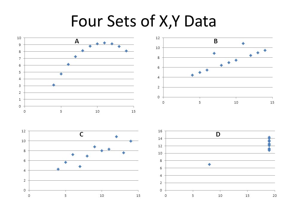
11. Data Set AData Set BData Set CData Set D XYXYXYXY 109.14108.04107.471912.08 88.1486.9586.471911.26 138.74137.58138.971913.21 98.7798.8196.971914.34 119.25118.331110.871913.97 148.1149.96149.471912.54 66.1367.2465.471910.75 43.144.2644.4787.00 129.131210.84128.471911.06 77.2674.8278.871913.41 54.7455.6854.971912.39 Four Sets of X,Y Data

13. SUMMARY OUTPUT Regression Statistics Multiple R0.8166 R Square0.6669 Adjusted R Square0.6299 Standard Error1.2357 Observations11 ANOVA dfSSMSFSignificance F Regression127.5100 18.01640.0022 Residual913.74251.5269 Total1041.2525 CoefficientsStandard Errort StatP-valueLower 95%Upper 95%Lower 95.0%Upper 95.0% Intercept2.99932.15321.39290.1971-1.87167.8702-1.87167.8702 X0.50010.11784.24460.00220.23360.76660.23360.7666 Four Sets of X,Y Data Data Analysis/Regression Identical Regression Output For A, B, C, and D!!!!!

14. Assumptions

15. Example: Section 4 IQs IQ Mean108.545 Standard Error3.448 Median110 Mode102 Standard Deviation19.807 Sample Variance392.318 Kurtosis0.228 Skewness-0.499 Range85 Minimum57 Maximum142 Sum3582 Count33 n s The CLT tells us this test works even if Y is not normal.

16. Regression Assumptions

17. Summary: The key assumption of linear regression….. Y ~ N(μ,σ) (no regression) Y│X ~ N(a+bX,σ) (with regression) – In other words μ = a + b (X) or E(Y│X) = a + b(X) Without regression, we used data to estimate and test hypotheses about the parameter μ. With regression, we use (x,y) data to estimate and test hypotheses about the parameters a and b. In both cases, we use the t because we don’t know σ. With regression, we also want to use X to forecast a new Y. The mean of Y given X is a linear function of X. EMBS (12.14)

18. Example: Assignment 22 MSFHours 262 34.24.17 294.42 34.34.75 85.94.83 143.26.67 85.57 140.67.08 140.67.17 40.47.17 10110 239.712 179.312.5 126.513.67 140.815.08 Regression Statistics Multiple R0.72600331 R Square0.527080806 Adjusted R Square0.490702407 Standard Error2.773595935 Observations15 ANOVA df Regression1 Residual13 Total14 Coefficients Intercept3.312316042 MSF0.044489502 n Standard error

19. Forecasting Y│X=157.3 Plug X=157.3 into the regression equation to get 10.31 as the point forecast. – The point forecast is the mean of the probability distribution forecast. Under Certain Assumptions……. – GOOD METHOD Pr(Y<8) = NORMDIST(8,10.31,2.77,true) = 0.202

20. Example: Assignment 22 MSFHours 262 34.24.17 294.42 34.34.75 85.94.83 143.26.67 85.57 140.67.08 140.67.17 40.47.17 10110 239.712 179.312.5 126.513.67 140.815.08 Regression Statistics Multiple R0.72600331 R Square0.527080806 Adjusted R Square0.490702407 Standard Error2.773595935 Observations15 ANOVA df Regression1 Residual13 Total14 Coefficients Intercept3.312316042 MSF0.044489502 Job AJob B Intercept11 MSF157.364.7 Point Forecast10.31056.1908 sigma2.77 X88 Normdist0.20210.7432 n Standard error

21. Forecasting Y│X=157.3 Plug X=157.3 into the regression equation to get 10.31 the point forecast. – The point forecast is the mean of the probability distribution forecast. Under Certain Assumptions……. – BETTER METHOD t= (8-10.31)/2.77 = -0.83 Pr(Y<8) = 1-t.dist.rt(-0.83,13) = 0.210 dof = n - 2

22. Forecasting Y│X=157.3 Plug X=157.3 into the regression equation to get 10.31 the point forecast. – The point forecast is the mean of the probability distribution forecast. Under Certain Assumptions……. – PERFECT METHOD t= (8-10.31)/2.93 = -0.79 Pr(Y<8) = 1-t.dist.rt(-0.79,13) = 0.222 dof = n - 2

23. Probability Forecasting with Regression summary

24. Probability Forecasting with Regression

25. Summed over the n data points The X for which we predict Y The good and better methods ignore these terms…okay the bigger the n. (EMBS 12.26)

26. BOTTOM LINE

27. Much ado about nothing? Perfect (widest and curved) Good (straight and narrowest) Better

28. TODAY Got a better idea of how the “least squares” regression line goes through the cloud of points. Saw that several “clouds” can have exactly the same regression line….so chart the cloud. Practiced using a regression equation to calculate a point forecast (a mean) Saw three methods for creating a probability distribution forecast of Y│X. – We will use the better method. – We will know that it understates the actual uncertainty…..a problem that goes away as n gets big.

29. Next Class We will learn about “adjusted R square” – (p 9-10 pfeifer note) – The most over-rated statistic of all time. We will learn the four assumptions required to use regression to make a probability forecast of Y│X. – (Section 5 pfeifer note, 12.4 EMBS) – And how to check each of them. We will learn how to test H0: b=0. – (p 12-13 pfeifer note, 12.5 EMBS) – And why this is such an important test.