1. Packet classification on Multiple Fields Authors: Pankaj Gupta and Nick McKcown Publisher: ACM 1999 Presenter: 楊皓中 Date: 2013/12/11

2. Introduction There are a number of network service that require packet classification,such as routing,access-control in firewalls, policy based routing. In each case, it is necessary to determine which flow an arriving packet belongs to so as to determine –for example— whether to forward or filter it, where to forward it to. We find that a simple multi-stage classification algorithm, call RFC(recursive flow classification)

3. Introduction

4. Proposed Algorithm RFC 一. Structure of the classifiers 二. Algorithm 三. A simple complete example of RFC

5. Structure of the classifiers

6. Algorithm

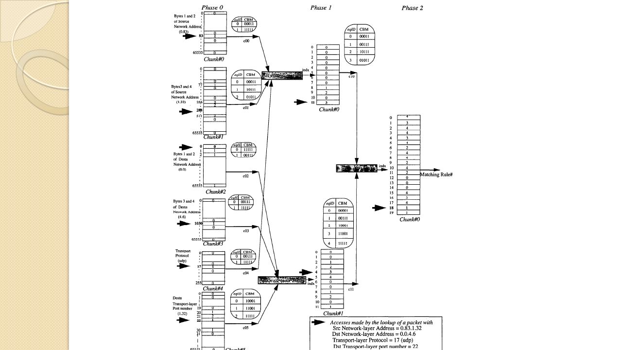
7. Algorithm 1) In the first phase, F fields of the packet header are split up into multiple chunks that are used to index into multiple memories in parallel. Each of the parallel lookups yields an output value that we will call eqlD 2) In subsequent phases, the index into each memory is formed by combining the results of the lookups from earlier phases. 3) In the final phase, we are left with one result from the lookup. Because of the way the memory contents have been pre-computed, this value corresponds to the classID of the packet.

9. Algorithm Example: Phase 0 table of chunk 6 ◦ 00 : {20,21} ◦ 01 : {www=80} ◦ 10 : {>1023} ◦ 11 : {all remaining number in 0-65535} ◦ two bit values the “equivalence classIDS” (eqIDs). ◦ CBM(class bitmap) ◦ Ex: Dport=20 ◦ http://www.arl.wustl.edu/~hs1/project/rfc.htm http://www.arl.wustl.edu/~hs1/project/rfc.htm indexeqID 03 13 |3 193 200 210 |3 793 801 813 |3 10233 10242 10253 |3 655353 eqIDCBM 0101000 1110100 2100011 3100000

10. Algorithm Example: Phase 0 table of chunk 4 ◦ 00 : {udp = 17} ◦ 01 : {tcp = 6} ◦ 10: {all remaining number in 0-255} ◦ Ex: dport =20,udp 02 |2 52 61 72 |2 162 170 182 |2 2552 indexeqID 03 13 |3 193 200 210 |3 793 801 813 |3 10233 10242 10253 |3 655353 indexeqID 00 11 21 32 43 51 61 74 81 91 101 111 eqIDCBM 0101000 1100000 2110000 3100100 4100011 eqIDCBM 0101000 1110100 2100011 3100000 eqIDCBM 0111000 1100111 2100000 indexeqID

12. RFC pre-processing The performance of RFC can be tuned with parameters P : ◦ For instance, two of the several possible reduction trees for P=3 and P=4 When there is more than one reduction tree possible for a given value of P, we choose a tree based on two heuristics: (i) we combine those chunks together which have the most “correlation” ◦ e.g. we combine the two 16-bit chunks of Network-layer source address in the earliest phase possible (ii) we combine as many chunks as we can without causing unreasonable memory consumption

13. RFC pre-processing Following these heuristics, we find that ◦ the “best” reduction tree for P=3 is tree-B in Figure 8 ◦ the “best” reduction tree for P=4 is tree-A in Figure 9. chunk 0source(32-16) 1source(15-0) 2destination(32-16) 3destination(15-0) 4protocol 5protocol-flags

14. RFC pre-processing Our first goal is to keep the total amount of memory reasonably small. The graphs show how the memory usage increases with the number of rules in each classifier P=2 P=3 P=4 small memory, but comes two additional memory access

15. as we increase the number of phases from three to four, we require a smaller total amount of memory. However, this comes at the expense of two additional memory accesses, illustrating the trade-off between memory consumption and lookup time in RFC

16. RFC pre-processing Our second goal is to keep the preprocessing time small. plot the preprocessing time required for both three and four phases of RFC The graphs indicate that, for these classifiers, RFC is suitable if the rules change relatively slowly; ◦ for example, not more than once every few seconds

17. RFC lookup performance

18. Adjacency Groups Since the size of the RFC tables depends on the number of chunk equivalence classes, ◦ we focus our efforts on trying to reduce this number. ◦ This we do by merging two or more rules of the original classifier. First, we define some notation. We call two distinct rules R and S. with R appearing first. in the classifier to be adjacent in dimension ‘I’ if all of the following three conditions hold: ◦ (1) They have the same action ◦ (2) All but the ‘I’ field have the exact same specification in the two rules ◦ (3) All rules appearing in between R and S in the classifier have either the same action or are disjoint from R. Two rules are said to be simply adjacent if they are adjacent in some dimension.

19. Adjacency Groups

20. Memory consumed with p=3with adjGrp

21. Comparison with other packet classification