1. KL-parameterization of atmospheric aerosol size distribution Hannes.Tammet@ut.ee University of Tartu, Institute of Physics with participation of Marko Vana Acknowledgements to Markku Kulmala and staff of Hyytiälä station KL parameterization of atmospheric aerosol size distribution 1. Assimilation of information 2. KL-model of size distribution 3. Test data 4. Test results

2. A well forgotten model, references: Tammet, H.F. (1988) Sravnenie model'nykh raspredeleniï aérozol'nykh chastits po razmeram (in Russian). Acta Comm. Univ. Tartu 824, 92–108. Translation of the previous paper: Tammet, H. (1992) Comparison of model distributions of aerosol particle sizes. Acta Comm. Univ. Tartu 947, 136–149, http://ael.physic.ut.ee/tammet/kl1992.pdf http://ael.physic.ut.ee/tammet/kl1992.pdf Tammet, H. (1988) Models of size spectrum of tropospheric aerosol. In Atmospheric Aerosols and Nucleation. Lecture Notes in Physics, Springer-Verlag, Vienna, 309, pp. 75–78, http://www.springerlink.com/content/p7l948j8m356605k http://www.springerlink.com/content/p7l948j8m356605k

3. An example: two parameterizations

4. Assimilation of information Correlated parameters a ja b Spread ~S1 Lost information: Spread ~S2

5. Theory: 2D lost information: Equivalent error amplification: nD lost information: Equivalent error amplification: correlation matrix correlation coefficient

6. KL-model of size distribution Modification from 1988/92 to 2012:  radius replaced by diameter,  natural logarithm replaced by decimal logarithm.

7. 3 variants of K

8. 3 variants of L

9. 3 variants of b

10. 3 variants of d x

11. Analytic properties

12. Test data: origin and preparation Hyytiälä aerosol measurements downloaded by Marko Vana Three full years of 2008, 2009 ja 2010 1107 files dmYYMMDD.sum 40-columns d = 3…983 nm 1051 files apsYYYYMMDD.sum 54-columns d = 523…19810 nm Time step 10 minutes, a file contains header and ja 144 lines of data. Some files contained broken lines or negative values of dn/dlgd, such files were rejected. Further, only these days were used where both DM and APS-files are present. Preparative operations:  DM & APS–files were joined using new logarithm-homogeneous fraction structure containing 62 fractions from 3 to 19110 nm (method – interpolation). Where both DM and APS data present the average was calculated using weights (d – 500) / 500 for APS and (1000 – d) / 500 for DMPS.  All diurnal files were merged into a single 3-year file while the time of an interval center was interpolated to sharp minute 5, 15, 25 … (using neighbors with deviation < 10.8 minutes).

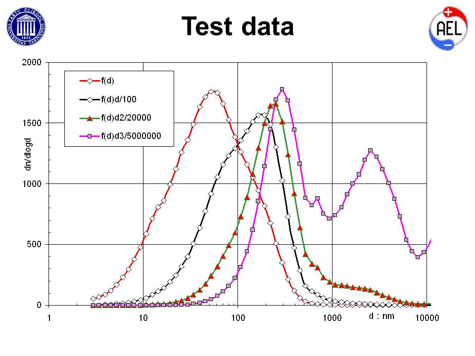
13. Test data The file of 10-minute records Hyytiala08-10aerosol.xl contains 62 data columns and 141367 data lines that is 89.6 % of the maximum 157824 10-minute intervals in the 3 years. The 10-minute data are pretty noisy. Next, the data were convereted to hourly averages. Only these hours were included that contain at least 3 measurements. The file of hourly averages Hyytiala08-10aerosol-h.xl contains one header line (incl. diameters) and 23517 data lines that cover 89.4% of possible 26304 hours. The 71 columns are: time DOY, 62 values of dn/dlgd, total number concentration, time parameters: year, month, day, hour, year quarter, day quarter, day-of-week.

14. Test data

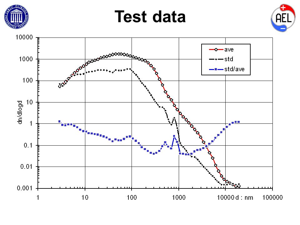
17. Some strange irregularities:  the interval 10…..165 nm contains dn/dlgd < 10 cm -3,  the interval 190…3000 nm contains dn/dlgd < 0.001 cm -3. Such hours were excluded from the final KL test data. The file of filtered hourly averages Hyytiala08-10aerosol-hf.xl (h = hours, f = filtered) contains 21682 hours that is 82.5% of possible maximum. Filtered test data

18. KL-parameterization of atmospheric aerosol size distribution TEST RESULTS

19. 3-year average: KL4 & KL5 from 10 to 3000 nm

20. What is KL5?

21. 3-year average: KL4 & KL5 from 3 to 10000 nm KL4: K = 3.18 L = 0.97 b = 4240 dx = 117 std = 0.152 KL5: K = 3.05 L = 1.01 b = 4980 dx = 98 c = 0.45 std = 0.138

22. Method of fitting Given: a table of function measured _dn/dlgd (d) Task: choose 5 parameters K L b d x c Special case of KL4  c = 0. The fitting deviation in typical diagrams is Δ = lg (fitted_dn/dlgd) – lg (measured_dn/dlgd). Measure of visual quality: std (Δ) Policy:  choose b so that average (Δ) = 0  choose other parameters so that std (Δ)  min. An arbitrary technique of minimization can be used

23. Fitting of test data Mean standard deviation between approximation and measurements of lg (dn/dlgd) KL4  0.192 KL5  0.144 Standard deviation of mean distribution approximation were: KL4  0.097 KL5  0.032

24. Examples: 10% of KL4 9500) 2009-04-14-12KL4: 0.109 3.681 0.265 1149 267 KL5: 0.106 3.616 0.229 1073 266 0.119

25. Examples: 10% of KL4 12752) 2009-09-30-05KL4 0.109 2.006 2.226 6407 18 KL5 0.094 2.000 2.446 6557 18 0.236

26. Examples: 10% of KL4 11805) 2009-08-19-07KL4 0.109 3.026 2.051 7109 70 KL5 0.108 2.924 2.33 7878 62 0.443

27. Examples: 50% of KL4 11714) 2009-08-11-10KL4 0.189 3.16 1.785 7544 114 KL5 0.095 2.795 2.353 9634 81 0.973

28. Examples: 50% of KL4 11844) 2009-08-20-23KL4 0.189 3.05 2.383 11169 55 KL5 0.189 3.044 2.403 11216 55 0.033

29. Examples: 50% of KL4 11915) 2009-08-24-04KL4 0.189 3.102 2.526 4226 95 KL5 0.102 2.855 2.982 4724 76 0.879

30. Examples: 90% of KL4 18557) 2010-08-11-13KL4 0.278 3.19 0.361 2101 163 KL5 0.172 2.663 0.745 3737 96 1.312

31. Examples: 90% of KL4 18549) 2010-08-11-05KL4 0.222 3.235 1.197 1472 154 KL5 0.182 2.615 1.954 2418 85 1.335

32. Examples: 90% of KL4 19310) 2010-09-14-12KL4 0.278 2.895 1.179 1293 104 KL5 0.120 2.523 2.127 2389 62 1.409

33. Analysis: KL4 Correlation matrix K L b d x 1.000 -0.251 -0.207 0.717 -0.251 1.000 0.594 -0.567 -0.207 0.594 1.000 -0.446 0.717 -0.567 -0.446 1.000 Det 0.191055, loss 0.36 digits, error amplification 1.23 Eigenvectors 0.449 0.666 -0.198 -0.561 -0.504 0.427 -0.668 0.340 -0.460 0.539 0.704 0.022 0.575 0.286 0.132 0.754 Eigenvalues 2.413 0.978 0.410 0.197

34. Analysis: KL5 Correlation matrix K L b d x c 1.000 -0.286 -0.152 0.730 -0.393 -0.286 1.000 0.589 -0.546 0.215 -0.152 0.589 1.000 -0.373 0.071 0.730 -0.546 -0.373 1.000 -0.336 -0.393 0.215 0.071 -0.336 1.000 Det 0.167549, loss 0.39 digits, error amplification 1.25 Eigenvectors 0.470 0.432 -0.422 -0.220 0.602 -0.473 0.418 -0.154 -0.699 -0.295 -0.377 0.619 -0.161 0.669 -0.017 0.553 0.125 -0.354 0.090 -0.737 -0.324 -0.487 -0.803 0.076 0.068 Eigenvalues 2.540 1.159 0.701 0.392 0.207

35. Conclusion: it works outx  graphic,  simple interpretation,  minimum loss of information,  analytic integrals available. Properties of KL:

36. 2009 THANK YOU, KL