1. Solar and Cosmic Ray Energetic Particle Models : Space Weather Aspects
Stephen B Gabriel
University of Southampton

2. Outline Effects What needs to be modelled/predicted Current Models
Future Directions
Conclusions
Dictionary Collins Concise
Prediction : the act of predicting;something predicted; a forecast
Predict : to state or make a declaration about in advance
Forecast :
To predict or calculate ( weather,events,etc), in advance
To serve as an early indication of
A statement of probable future weather calculated from meteoroligal data
A prediction
Weather : 1 the day to day meteorological conditions affecting a specific place

3. What needs to be predicted
For all high energy particle species(electrons, protons and heavy ions):
Flux spectrum ( instantaneous)
Fluence spectrum
Directionality
Spatial dependence
At any time ( including solar cycle variations)

4. Model Requirements Time scales Fidelity(Accuracy) Lead time Yes/No
Average(Longer time)
Fidelity(Accuracy)
False Alarm Rates

7. “Bastille Day Event” (July 14th 2000) Sampling: 5 minutes

8. Current Models Galactic Cosmic Rays (GCR) :
Creme 96 (semi-empirical, uses Nymmik’s solar cycle modulation)
Solar Energetic Particle Events (SEPE)
Protons : Heavy Ions :
JPL-91 * Tylka
Xapsos
Nymmik
Rosenqvist and Hilgers

9. GCR Models
CREME 96 regarded as the most up-to-date and comprehensive model
CREME96 is an update of the Cosmic Ray Effects on Micro-Electronics code, a widely-used suite of programs for creating numerical models of the ionizing-radiation environment in near-Earth orbits and for evaluating radiation effects in spacecraft.

10. CREME 96 Has many significant features, including
(1) improved models of the galactic cosmic ray, anomalous cosmic ray, and solar energetic particle components of the near-Earth environment;
(2) improved geomagnetic transmission calculations;
(3) improved nuclear transport routines;
(4) improved single-event upset (SEU) calculation techniques, for both proton-induced and direct-ionization-induced SEUs; and
(5) an easy-to-use graphical interface, with extensive on-line tutorial information.

11. CREME 96 Also includes 3 levels of solar particle intensities
Worst week model ( based on SEP fluxes averaged over 180 hrs ( 7.5 days beginning 1300 UT on 19 October 1989) ~ 99% worst case
Worst day model SEP fluxes averaged over 18 hours beginning 1300 UT on 20 October 1989
Peak Flux model : based on the peak 5 minute fluxes observed on GOES in October 1989

12. Cosmic Rays: Solar Cycle Modulation CREME 96

13. GCR Short term variations : 27 day periodicity Forbush decreases
Caused by CMEs
Various physics based models (worldwide)
No predictive model available

14. Fluence Probability Curve

15. SEPE Predictive Models
2 types :
Short lead time ~ hours ( more or less based on the detection of another event close to start of the SEPE)(SEC,Dorman and others,Sanahuja (SOLPENCO) and others)
Longer term ( ~> 24hours) (Neural Networks)

16. Comparison with SEC PROTONS
SEC PROTONS: ~6hour lead time
PROTONS (for year of 1989)
79% Overall Success
~6 Hour lead time
Neural Model
65% Overall Success
48 Hour lead time
16% lower accuracy
Order of magnitude gain in lead time
Neural Model: 48hour lead time

17. Geomagnetic Shielding
Models available :
Stormer Theory
Magnetocosmics (Flückiger et al)
Atmocosmics (Flückiger et al)

20. Future Modelling Directions
GCR :
Improved accuracy of long term variations ( on solar cycle time scales) (eg CREME 96)
Predictive modelling of Forbush decreases
Importance of partially-ionised heavy ions (mean-ionic charge ~14 rather than 26)
SEPE :
Statistical :
More data( real and simulated)!
Solar minimum
Solar cycle variations
Heliospheric radial variations of flux and fluence
Better spectral modelling

21. Future Modelling Directions(cont.)
SEPE :
Predictive
Longer lead times ? Better specification of requirements from users
Use of neural networks with more ‘intelligent’ inputs – pre-processing of data; more( simulated data?)
Wavelets
More testing of models leading towards an operational model

22. Conclusions Paucity of data for SEPE
Lack of complete understanding of underlying physics of SEPE
Need for better understanding of SEPE and geomagnetic storms occurring simultaneously ( depression of geomagnetic cut-off and formation of new trapped radiation belt protons)
All models semi-empirical physics models will take at least 5 years to develop

24. Conclusions 
Concentrated on existing engineering models and their inadequacies,ideally what is needed and some of the basic physics
Models :
Cosmic Rays: CREME 96: 
Uses Nymmik's semi-empirical model for solar cycle modulation based on Wolf sunspot number (includes large-scale structure of heliospheric magnetic field)
Incorporates multiply-charged ACR component (above ~ 20 MeV/nucleon), from Sampex results
~ 25% error on average for solar modulation and spectra, compared to data

25. Conclusions (contd.)  Geomagnetic Shielding
Solar Protons 
More data analysis/modelling during active periods to understand cut-off depression/predict transmission (CRÈME 96 combined IGRF and extended Tsyganenko model)
Importance of partially-ionised heavy ions
(mean-ionic charge ~14 rather than 26)
Better understanding of formation of new trapped belt

26. Short–term SEPE Models An Example
Prediction ability
SEC ‘PROTONS’ and Garcia models
Require an x-ray flare
Physically limited lead time
No prediction capability for lead times > ~6hours

28. Effects

29. Comparison of 3 Models
Nymmik assumes that the mean event frequency is proportional to the average sunspot number while others assume that there are 7 active years of a solar cycle
JPL models assume a log normal distribution, Xapsos uses maximum entropy method to get best distribution function( truncated power law) while Nymmik model assumes a power law
JPL model only goes up to >60MeV, MSU model up to 100s of MeV and Xapsos > 300MeV

30. Comparison of 3 Models
JPL model is for fluences only while MSU and Xapsos have peak flux models too
Event definition appears to be different between JPL and MSU models
Different data sets for all three models

31. Types of Models Physical Empirical/Statistical
Engineering ( different from empirical)
Boundaries – stop at edge of magnetosphere?

32. SEPE models Statistical/probabilistic models :
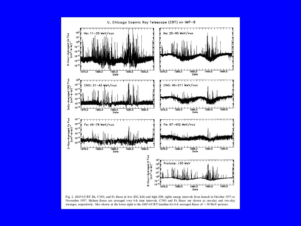
4 most recent proton models :
JPL – 91
Xapsos et al
Nymmik(MSU)
Hilgers et al
Heavy Ion Model : Tylka :
‘Probability Distributions of High-energy Solar Heavy-Ion Fluxes from IMP-8: ’
IEEE Transactions on Nuclear Science,
VOL. 44, NO. 6, December 1997

33. What is needed to predict SEPEs – Deterministic (Physics Based)
A complete understanding of the underlying physical mechanisms that cause SEPEs
Currently , it is generally accepted that CMEs and shocks play a key role
In principle if we knew the conditions on the sun ( and in interplanetary space) that caused these CMEs and shocks then could predict the SEPEs
Recent results from SOHO(UV/EUV( UVCS, EIT),CMEs(LASCO),etc) and other solar observatories (e.g Yohkoh)have done much to increase our understanding