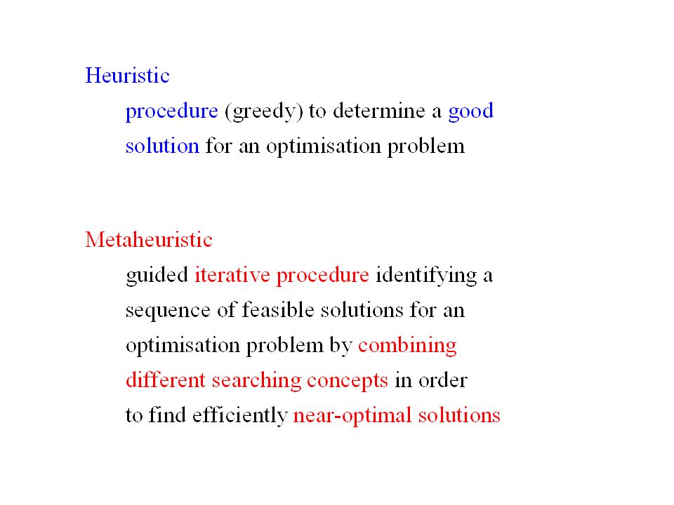
1. METAHEURISTIC Jacques A. Ferland Department of Informatique and Recherche Opérationnelle Université de Montréal ferland@iro.umontreal.ca www.iro.umontreal.ca/~ferland/ March 2015

2. Introduction Introduction to some basic methods My vision relying on my experience Not an exaustive survey Most of the time ad hoc adaptations of basic methods are used to deal with specific applications

4. Advantages of using metaheuristic Intuitive and easy to understand With regards to enduser of a real world application: - Easy to explain - Connection with the manual approach of enduser - Enduser sees easily the added features to improve the results - Allow to analyze more deeply and more scenarios Allow dealing with larger size problems having higher degree of complexity Generate rapidly very good solutions

5. Disadvantages of using metaheuristic Quick and dirty methods Optimality not guaranted in general Few convergence results for special cases

6. Overview Heuristic Constructive Techniques: Generate a good solution Local (Neighborhood) Search Methods (LSM): Iterative procedure improving a solution Population-based Methods: Population of solutions evolving to mimic a natural process

7. Preliminary: Problems used to illustrate General problem Assignment type problem: Assignment of resources j to activities i

8. Problem Formulation Assignment type problem Graph coloring problem : Graph G = (V,E). V = { i : 1≤ i ≤ n} ; E = {(i, l) : (i, l) edge of G}. Set of colors {j : 1≤ j ≤ m}

9. Graph coloring example Graph coloring problem : Graph G = (V,E). V = { i : 1≤ i ≤ n} ; E = {(i, l) : (i, l) edge of G}. Set of colors {j : 1≤ j ≤ m} The following encoding of a solution x is interesting for solving the graph coloring problem: x => where for each vertex i,

10. Heuristic Constructive Techniques Greedy GRASP (Greedy Randomized Adaptive Search Procedure)

11. Heuristic Constructive Techniques Values of the variables are determined sequentially: at each iteration, a variable is selected, and its value is determined The value of each variable is never modifided once it is determined Techniques often used to generate initial solutions for iterative procedures

12. Greedy method Next variable to be fixed and its value are selected to optimize the objective function given the values of the variables already fixed Graph coloring problem: Vertices are ordered in decreasing order of their degree Vertices selected in that order For each vertex, select a color in order to reduce the number of pairs of adjacent vertices already colored with the same color

13. Graph coloring example Graph with 5 vertices 2 colors available: red blue

14. Graph coloring example Vertices in decreasing order of degree Vertex degree color 2 3 1 2 3 2 4 2 5 1

15. Graph coloring example Vertices in decreasing order of degree Vertex degree color 2 3 1 2 3 2 4 2 5 1 Vertex 2 color number of adj. vert. same color red 0 blue 0 <=

16. Graph coloring example Vertices in decreasing order of degree Vertex degree color 2 3 blue 1 2 3 2 4 2 5 1 Vertex 2 color number of adj. vert. same color red 0 blue 0 <=

17. Graph coloring example Vertices in decreasing order of degree Vertex degree color 2 3 blue 1 2 3 2 4 2 5 1

18. Graph coloring example Vertices in decreasing order of degree Vertex degree color 2 3 blue 1 2 3 2 4 2 5 1 Vertex 1 color number of adj. vert. same color red 0 <= blue 1

19. Graph coloring example Vertices in decreasing order of degree Vertex degree color 2 3 blue 1 2 red 3 2 4 2 5 1 Vertex 1 color number of adj. vert. same color red 0 <= blue 1

20. Graph coloring example Vertices in decreasing order of degree Vertex degree color 2 3 blue 1 2 red 3 2 4 2 5 1

21. Graph coloring example Vertices in decreasing order of degree Vertex degree color 2 3 blue 1 2 red 3 2 4 2 5 1 Vertex 3 color number of adj. vert. same color red 1 <= blue 1

22. Graph coloring example Vertices in decreasing order of degree Vertex degree color 2 3 blue 1 2 red 3 2 red 4 2 5 1 Vertex 3 color number of adj. vert. same color red 1 <= blue 1

23. Graph coloring example Vertices in decreasing order of degree Vertex degree color 2 3 blue 1 2 red 3 2 red 4 2 5 1

24. Graph coloring example Vertices in decreasing order of degree Vertex degree color 2 3 blue 1 2 red 3 2 red 4 2 5 1 Vertex 4 color number of adj. vert. same color red 0 <= blue 1

25. Graph coloring example Vertices in decreasing order of degree Vertex degree color 2 3 blue 1 2 red 3 2 red 4 2 red 5 1 Vertex 4 color number of adj. vert. same color red 0 <= blue 1

26. Graph coloring example Vertices in decreasing order of degree Vertex degree color 2 3 blue 1 2 red 3 2 red 4 2 red 5 1

27. Graph coloring example Vertices in decreasing order of degree Vertex degree color 2 3 blue 1 2 red 3 2 red 4 2 red 5 1 Vertex 5 color number of adj. vert. same color red 1 blue 0 <=

28. Graph coloring example Vertices in decreasing order of degree Vertex degree color 2 3 blue 1 2 red 3 2 red 4 2 red 5 1 blue Vertex 5 color number of adj. vert. same color red 1 blue 0 <=

29. GRASP Greedy Randomized Adaptive Search Procedure Next variable to be fixed is selected randomly among those inducing the smallest increase. Referring to the general problem, i) let J’ = { j : x j is not fixed yet} and δ j be the increase induces by the best value that x j can take ( j є J’ ) ii) Denote and α є [0, 1]. iii) Select randomly j’ є {j є J’ : δ j ≤ ( 1 / α ) δ* } and fix the value of x j’

30. Graph coloring example Graph with 5 vertices 2 colors available: red blue α = 0.5

31. Graph coloring example Vertex j best color δ j color 1 any 0 2 any 0 3 any 0 4 any 0 5 any 0

32. Graph coloring example Vertex j best color δ j color 1 any 0 2 any 0 3 any 0 4 any 0 5 any 0 J’ = {1, 2, 3, 4, 5} δ* = 0 α = 0.5 {j є J’ : δ j ≤ ( 1 / α ) δ* }= {1, 2, 3, 4, 5}  Select randomly vertex 3 color blue

33. Graph coloring example Vertex j best color δ j color 1 any 0 2 any 0 3 any 0 blue 4 any 0 5 any 0 J’ = {1, 2, 3, 4, 5} δ* = 0 α = 0.5 {j є J’ : δ j ≤ ( 1 / α ) δ* }= {1, 2, 3, 4, 5}  Select randomly vertex 3 color blue

34. Graph coloring example Vertex j best color δ j color 1 red 0 2 red 0 3 blue 4 any 0 5 any 0

35. Graph coloring example Vertex j best color δ j color 1 red 0 2 red 0 3 blue 4 any 0 5 any 0 J’ = {1, 2, 4, 5} δ* = 0 α = 0.5 {j є J’ : δ j ≤ ( 1 / α ) δ* }= {1, 2, 4, 5}  Select randomly vertex 4 color red

36. Graph coloring example Vertex j best color δ j color 1 red 0 2 red 0 3 blue 4 any 0 red 5 any 0 J’ = {1, 2, 4, 5} δ* = 0 α = 0.5 {j є J’ : δ j ≤ ( 1 / α ) δ* }= {1, 2, 4, 5}  Select randomly vertex 4 color red

37. Graph coloring example Vertex j best color δ j color 1 red 0 2 any 1 3 blue 4 red 5 blue 0

38. Graph coloring example Vertex j best color δ j color 1 red 0 2 any 1 3 blue 4 red 5 blue 0 J’ = {1, 2, 5} δ* = 0 α = 0.5 {j є J’ : δ j ≤ ( 1 / α ) δ* }= {1, 5}  Select randomly vertex 5 color blue

39. Graph coloring example Vertex j best color δ j color 1 red 0 2 any 1 3 blue 4 red 5 blue 0 blue J’ = {1, 2, 5} δ* = 0 α = 0.5 {j є J’ : δ j ≤ ( 1 / α ) δ* }= {1, 5}  Select randomly vertex 5 color blue

40. Graph coloring example Vertex j best color δ j color 1 red 0 2 any 1 3 blue 4 red 5 blue

41. Graph coloring example Vertex j best color δ j color 1 red 0 2 any 1 3 blue 4 red 5 blue J’ = {1, 2} δ* = 0 α = 0.5 {j є J’ : δ j ≤ ( 1 / α ) δ* }= {1}  Select vertex 1 color red

42. Graph coloring example Vertex j best color δ j color 1 red 0 red 2 any 1 3 blue 4 red 5 blue J’ = {1, 2} δ* = 0 α = 0.5 {j є J’ : δ j ≤ ( 1 / α ) δ* }= {1}  Select vertex 1 color red

43. Graph coloring example Vertex j best color δ j color 1 red 2 blue 1 3 blue 4 red 5 blue

44. Graph coloring example Vertex j best color δ j color 1 red 2 blue 1 3 blue 4 red 5 blue J’ = {2} δ* = 1 α = 0.5 {j є J’ : δ j ≤ ( 1 / α ) δ* }= {2}  Select vertex 2 color blue

45. Graph coloring example Vertex j best color δ j color 1 red 2 blue 1 blue 3 blue 4 red 5 blue J’ = {2} δ* = 1 α = 0.5 {j є J’ : δ j ≤ ( 1 / α ) δ* }= {2}  Select vertex 2 color blue

46. Graph coloring example Vertex j best color δ j color 1 red 2 blue 3 blue 4 red 5 blue J’ = Φ

48. Local(Neighborhood) Search Methods (LSM) A Local (Neighborhood) Search Method (LSM) is an iterative procedure starting with an initial feasible solution x 0. At each iteration: - we move from the current solution to a new one in its neighborhood N(x) - becomes the current solution for the next iteration - we update the best solution x* found so far. The procedure continues until some stopping criterion is satisfied

49. Local(Neighborhood) Search Methods (LSM) Descent (D) Tabu Search (TS) Simulated Annealing (SA) Improving strategies - Intensification - Diversification Variable Neighborhood Search (VNS) Exchange Procedure (EP) Adaptive Large Neighborhood Search (ALNS)

50. Neighborhood Neighborhood N(x) : The neighborhood N(x) varies with the problem, but its elements are always generated by slightly modifying x. If we denote M the set of modifications (or moves) to generate neighboring solutions, then N(x) = {x' : x' = x  m, m  M }

51. Neighborhood for assignment type problem The elements of the neighborhood N(x) are generated by slightly modifying x: N(x) = {x' : x' = x  m, m  M }

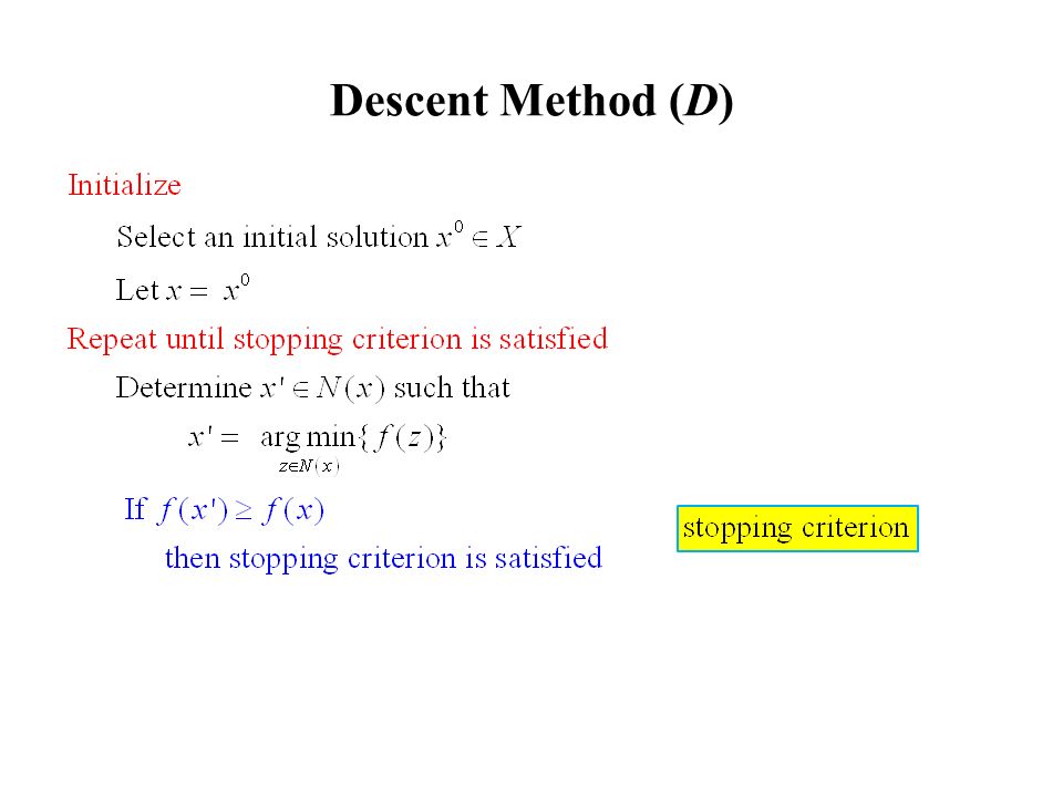
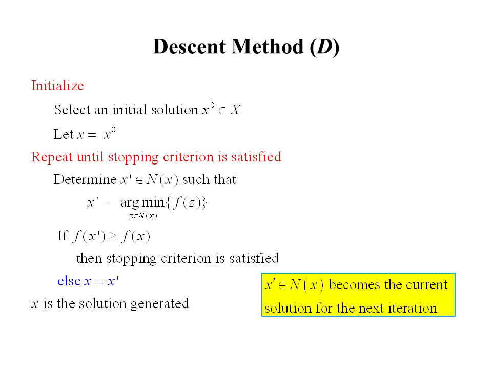
52. Descent Method (D) At each iteration, a best solution is selected as the current solution for the next iteration. Stopping criterion: f(x') ≥ f(x) i.e., the current solution cannot be improved or a first local minimum is reached.

53. Descent Method (D)

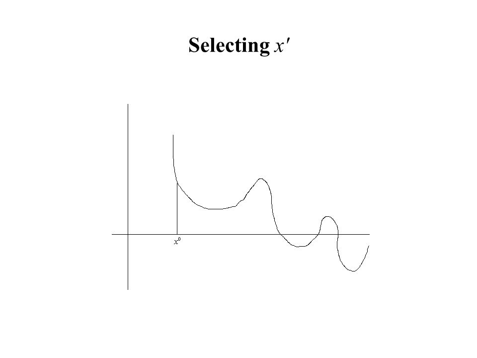
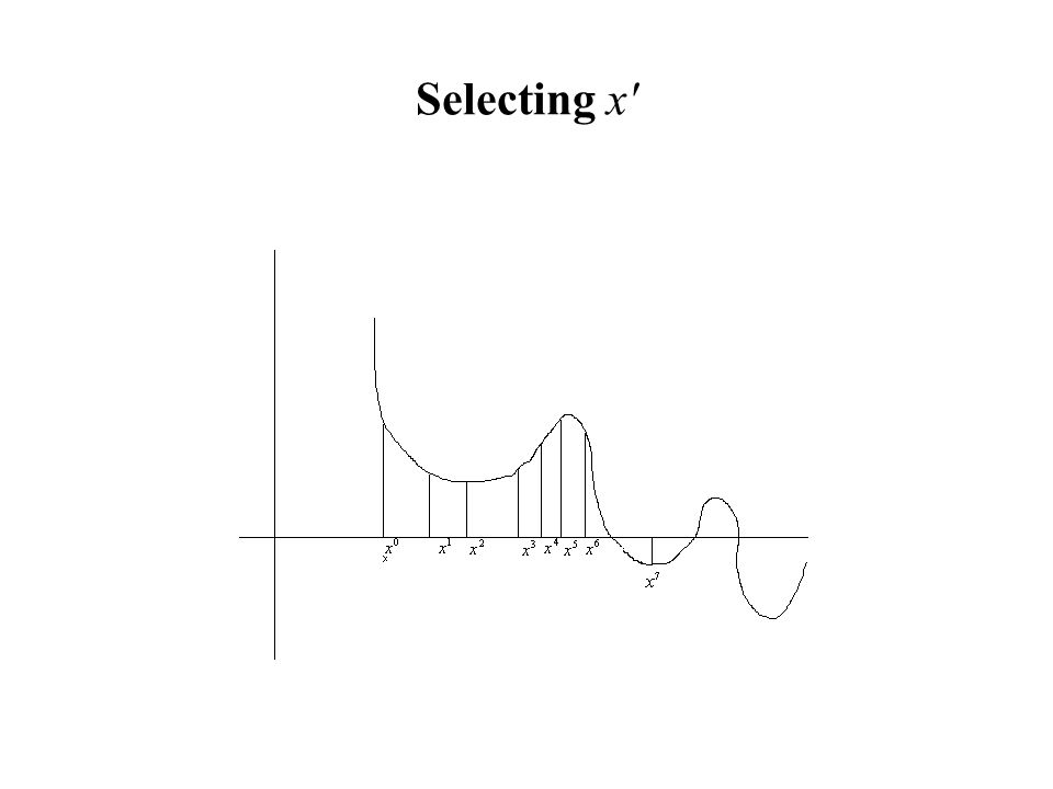
57. Selecting x'

61. Knapsack Problem Problem formulation: max f(x) = 18x 1 + 25x 2 + 11x 3 + 14x 4 Subject to 2x 1 + 2x 2 + x 3 + x 4 ≤ 3 (*) x 1, x 2, x 3, x 4 = 0 or 1. Neighborhood N(x) specified by the following modification or move: The value of one and only one variable is modified (from 0 to 1 or from 1 to 0) to generate a new solution satisfying constraint 2x 1 + 2x 2 + x 3 + x 4 ≤ 3 (*)

62. Knapsack Problem Initial sol. x 0 = x = [1, 0, 0, 0] ; f(x) = 18 N(x) f [0, 0, 0, 0] 0 [1, 0, 1, 0] 29 [1, 0, 0, 1] 32

63. Knapsack Problem Initial sol. x 0 = x = [1, 0, 0, 0] ; f(x) = 18 N(x) f [0, 0, 0, 0] 0 [1, 0, 1, 0] 29 [1, 0, 0, 1] 32 x' = [1, 0, 0, 1] ; f(x') = 32 Since f(x') >f(x), then x' replaces the current sol. x and we start a new iteration

64. Knapsack Problem current sol. x = [1, 0, 0, 1] ; f(x) = 32 N(x) f [0, 0, 0, 1] 14 [1, 0, 0, 0] 18

65. Knapsack Problem Current sol. x = [1, 0, 0, 1] ; f(x) = 32 N(x) f [0, 0, 0, 1] 14 [1, 0, 0, 0] 18 x' = [1, 0, 0, 0] ; f(x') = 18 Since f(x') < f(x), then the procedure stops with x* = x

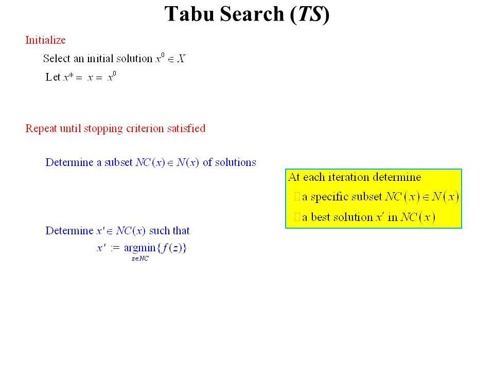
66. Tabu Search (TS) Tabu Search is an iterative neighborhood or local search technique At each iteration we move from a current solution x to a new solution x' in a neigborhood N(x) of x, until we reach some solution x* acceptable according to some criterion

67. Tabu Search (TS)

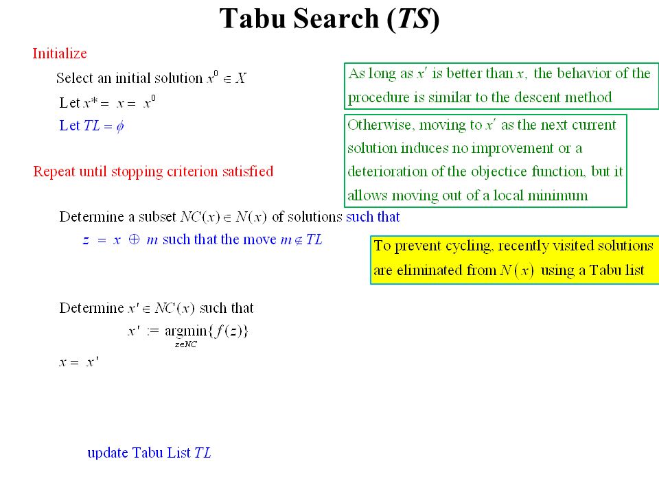
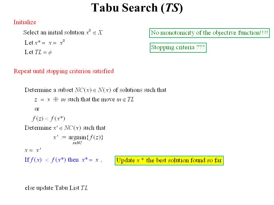
71. Tabu Lists (TL) Short term Tabu list TL is used to remember attributes or characteristics of the modification used to generate the new current solution A Tabu List often used for the assignment type problem is the following: If the new current solution x' is generated from x by modifying the resource of i from j(i) to p, then the pair (i, j(i)) is introduced in the Tabu list TL If the pair (i, j) is in TL, then any solution where resource j is to be assigned to i is declared Tabu The Tabu list is cyclic in order for an attribute to remain Tabu for a fixed number k of iterations

72. Tabu Search (TS)

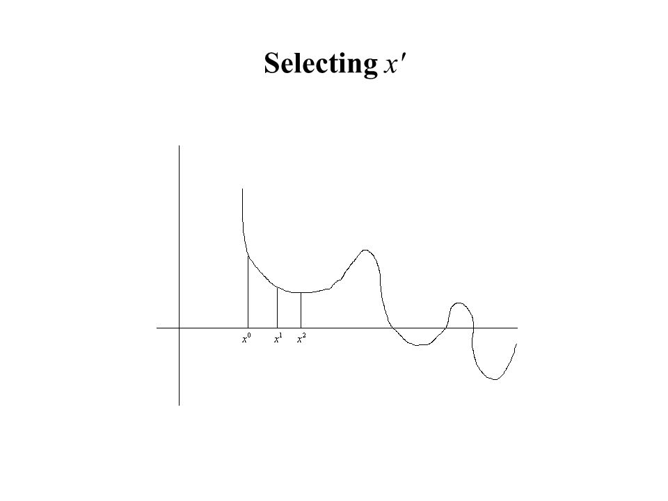
75. Selecting x'

82. Knapsack Problem Problem formulation: max f(x) = 18x 1 + 25x 2 + 11x 3 + 14x 4 Subject to 2x 1 + 2x 2 + x 3 + x 4 ≤ 3 x 1, x 2, x 3, x 4 = 0 or 1. Neighborhood N(x) specified by the following modification or move: The value of one and only one variable is modified (from 0 to 1 or from 1 to 0) to generate a new solution satisfying constraint Tabu list TL : element introduced in the Tabu list is the pair (index of modified variable, current value of the modified variable) Length of Tabu list = 2 itermax = 5 nitermax = 4

83. Knapsack Problem TL = Φ iter = 1 niter = 1 Initial sol. x 0 = x = [1, 0, 0, 0] ; f(x) = 18 N(x) f [0, 0, 0, 0] 0 [1, 0, 1, 0] 29 [1, 0, 0, 1] 32

84. Knapsack Problem Initial sol. x 0 = x = x* = [1, 0, 0, 0] ; f(x) = 18 N(x) f [0, 0, 0, 0] 0 [1, 0, 1, 0] 29 [1, 0, 0, 1] 32 x' = [1, 0, 0, 1] ; f(x') = 32 Since f(x') > f(x*) = 18, then x* = x', and niter := 0 x' replaces the current sol. x and we start a new iteration TL = { (4, 0)} Tabu list = Φ iter = 1 niter = 1

85. Knapsack Problem Current sol. x = [1, 0, 0, 1] ; f(x) = 32 N(x) f [0, 0, 0, 1] 14 [1, 0, 0, 0] 18 <= tabu TL = { (4, 0)} iter = 2 niter = 1

86. Knapsack Problem Current sol. x = [1, 0, 0, 1] ; f(x) = 32 N(x) f [0, 0, 0, 1] 14 [1, 0, 0, 0] 18 <= tabu x' = [0, 0, 0, 1] ; f(x') = 14 Since f(x') < f(x*) = 32, then x* not modified x' replaces the current sol. x and we start a new iteration TL = { (4, 0), (1, 1)} TL = { (4, 0)} iter = 2 niter = 1

87. Knapsack Problem Current sol. x = [0, 0, 0, 1] ; f(x) = 14 N(x) f [1, 0, 0, 1] 32 <= tabu [0, 1, 0, 1] 39 [0, 0, 1, 1] 25 [0, 0, 0, 0] 0 <= tabu TL = { (4, 0), (1, 1)} iter = 3 niter = 2

88. Knapsack Problem Current sol. x = [0, 0, 0, 1] ; f(x) = 14 N(x) f [1, 0, 0, 1] 32 <= tabu [0, 1, 0, 1] 39 [0, 0, 1, 1] 25 [0, 0, 0, 0] 0 <= tabu x' = [0, 1, 0, 1] ; f(x') = 39 Since f(x') > f(x*) = 32, then x* = x', and niter := 0 x' replaces the current sol. x and we start a new iteration TL = { (1, 1), (2, 0)} TL = { (4, 0), (1, 1)} iter = 3 niter = 2

89. Knapsack Problem Current sol. x = [0, 1, 0, 1] ; f(x) = 39 N(x) f [0, 0, 0, 1] 14 <= tabu [0, 1, 0, 0] 25 TL = { (1, 1), (2, 0)} iter = 4 niter =1

90. Knapsack Problem. Current sol. x = [0, 1, 0, 1] ; f(x) = 39 N(x) f [0, 0, 0, 1] 14 <= tabu [0, 1, 0, 0] 25 x' = [0, 1, 0, 0] ; f(x') = 25 Since f(x') < f(x*) = 39, then x* is not modified x' replaces the current sol. x and we start a new iteration TL = { (2, 0), (4, 1)} TL = { (1, 1), (2, 0)} iter = 4 niter =1

91. Knapsack Problem TL = { (2, 0), (4, 1)} iter = 5 niter =2 Stop since iter = itermax = 5 The solution x* = [0, 1, 0, 1] f(x*) = 39

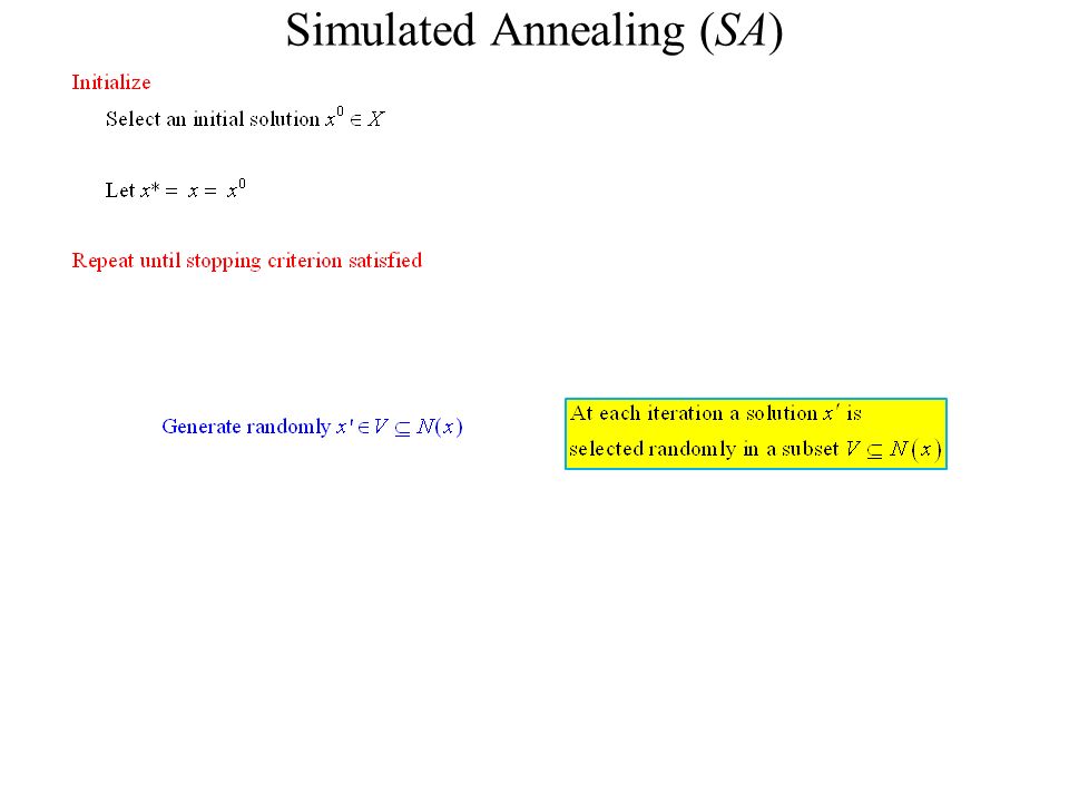
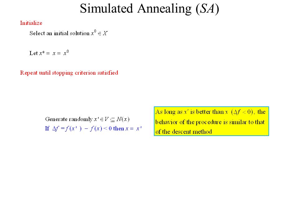
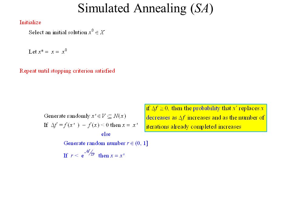
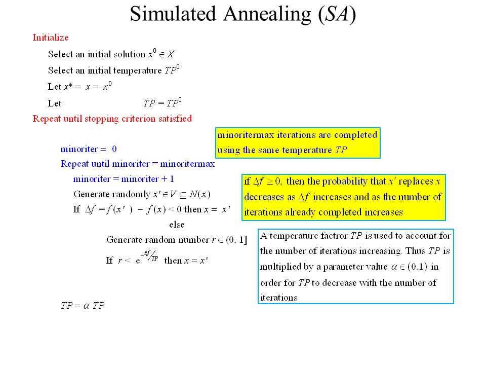
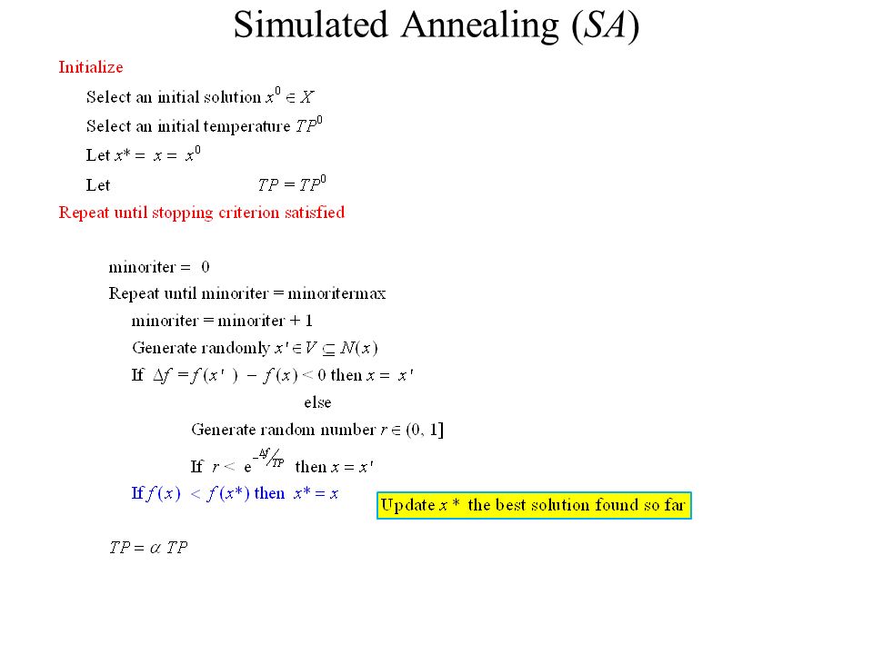
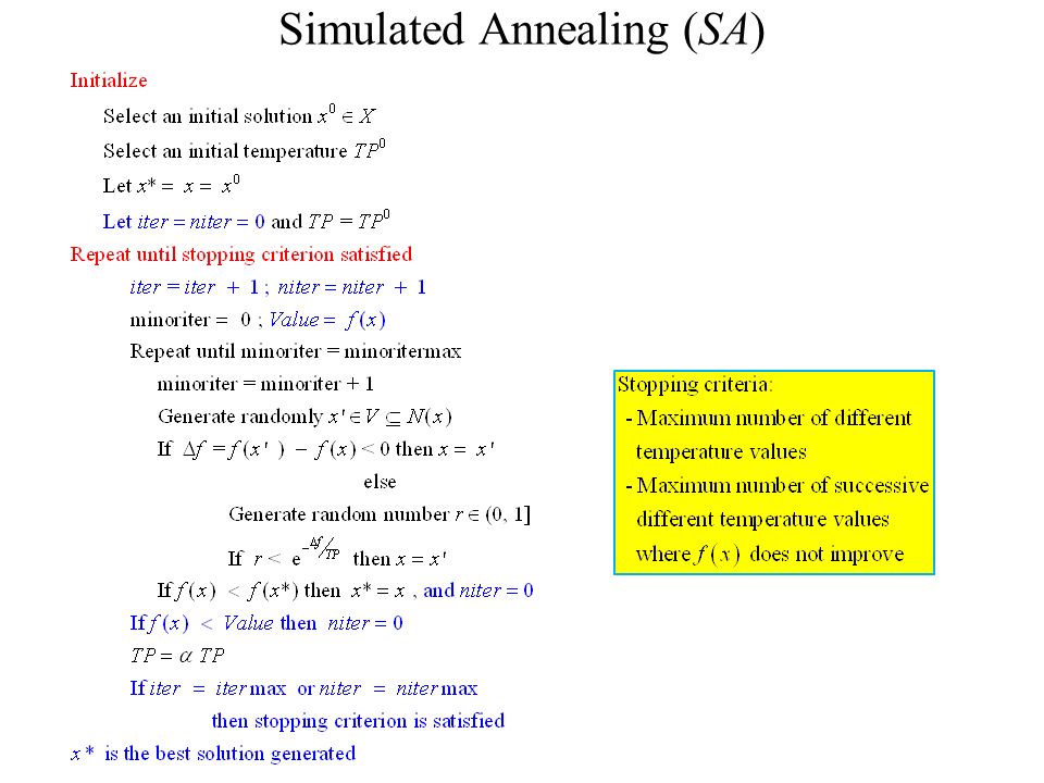
92. Simulated Annealing (SA) Probabilistic technique allowing to move out of local minima At each iteration, a solution x' is selected randomly in a subset of the neighborhood N(x) This approach was already used to simulate the evolution of an unstable physical system toward a thermodynamic stable equilibrium point at a fixed temperature

93. Simulated Annealing (SA)

101. Knapsack Problem Problem formulation: max f(x) = 18x 1 + 25x 2 + 11x 3 + 14x 4 Subject to 2x 1 + 2x 2 + x 3 + x 4 ≤ 3 x 1, x 2, x 3, x 4 = 0 or 1. Neighborhood N(x) specified by the following modification or move: The value of one and only one variable is modified (from 0 to 1 or from 1 to 0) to generate a new solution satisfying constraint 2x 1 + 2x 2 + x 3 + x 4 ≤ 3 TP 0 = 20 α = 0.5 itermax = 3 minoritermax = 2 nitermax = 2

102. Knapsack Problem Random numbers sequence: 0.55 0.72, 0.83, 0.55, 0.41, 0.09, 0.64 Initial sol. x 0 = x = [1, 0, 0, 0] ; f(x) = 18 ; Value = 18 N(x) f [0, 0, 0, 0] 0 [1, 0, 1, 0] 29 [1, 0, 0, 1] 32 TP = 20 iter = 1 minoriter = 1 niter = 1

103. Knapsack Problem max f(x) = 18x 1 + 25x 2 + 11x 3 + 14x 4 Subject to 2x 1 + 2x 2 + x 3 + x 4 ≤ 3 x 1, x 2, x 3, x 4 = 0 or 1. Random number : 0.72 TP = 20 iter = 1 minoriter = 1 niter = 1 Initial sol. x 0 = x = [1, 0, 0, 0] ; f(x) = 18 ; Value = 18 N(x) f [0, 0, 0, 0] 0 [1, 0, 1, 0] 29 [1, 0, 0, 1] 32 [0, 0, 0, 0] [1, 0, 1, 0] [1, 0, 0, 1] 0.33.66 1.72 x' = [1, 0, 0, 1] ; f(x') = 32

104. Knapsack Problem max f(x) = 18x 1 + 25x 2 + 11x 3 + 14x 4 Subject to 2x 1 + 2x 2 + x 3 + x 4 ≤ 3 x 1, x 2, x 3, x 4 = 0 or 1. Random number : 0.72 TP = 20 iter = 1 minoriter = 1 niter = 1 Initial sol. x 0 = x = [1, 0, 0, 0] ; f(x) = 18 ; Value = 18 N(x) f [0, 0, 0, 0] 0 [1, 0, 1, 0] 29 [1, 0, 0, 1] 32 [0, 0, 0, 0] [1, 0, 1, 0] [1, 0, 0, 1] 0.33.66 1.72 x' = [1, 0, 0, 1] ; f(x') = 32 Since f(x') > f(x) = 18, then x' replaces the current sol. x

105. Knapsack Problem max f(x) = 18x 1 + 25x 2 + 11x 3 + 14x 4 Subject to 2x 1 + 2x 2 + x 3 + x 4 ≤ 3 x 1, x 2, x 3, x 4 = 0 or 1. Random numbers sequence: 0.55 0.72, 0.83, 0.55, 0.41, 0.09, 0.64 Sol. x = [1, 0, 0, 1] ; f(x) = 32 ; Value = 18 N(x) f [0, 0, 0, 1] 14 [1, 0, 0, 0] 18 TP = 20 iter = 1 minoriter = 2 niter = 1

106. Knapsack Problem max f(x) = 18x 1 + 25x 2 + 11x 3 + 14x 4 Subject to 2x 1 + 2x 2 + x 3 + x 4 ≤ 3 x 1, x 2, x 3, x 4 = 0 or 1. Random number : 0.83 0.72, 0.83 TP = 20 iter = 1 minoriter = 2 niter = 1 Sol. x = [1, 0, 0, 1] ; f(x) = 32 ; Value = 18 N(x) f [0, 0, 0, 1] 14 [1, 0, 0, 0] 18 [0, 0, 0, 1] [1, 0,0, 0] 0 0.5 1 0.83 x' = [1, 0, 0, 0] ; f(x') = 18

107. Knapsack Problem max f(x) = 18x 1 + 25x 2 + 11x 3 + 14x 4 Subject to 2x 1 + 2x 2 + x 3 + x 4 ≤ 3 x 1, x 2, x 3, x 4 = 0 or 1. Random number: 0.55 0.72, 0.83, 0.55, 0.41, 0.09, 0.64 TP = 20 iter = 1 minoriter = 2 niter = 1 Sol. x = [1, 0, 0, 1] ; f(x) = 32 ; Value = 18 N(x) f [0, 0, 0, 1] 14 [1, 0, 0, 0] 18 [0, 0, 0, 1] [1, 0,0, 0] 0 0.5 1 0.83 x' = [1, 0, 0, 0] ; f(x') = 18 ∆f = 18 – 32 = - 14 Since e - 14 / 20 ≈ 0.497 < 0.55 we keep the same current solution x

108. Knapsack Problem max f(x) = 18x 1 + 25x 2 + 11x 3 + 14x 4 Subject to 2x 1 + 2x 2 + x 3 + x 4 ≤ 3 x 1, x 2, x 3, x 4 = 0 or 1. Random numbers sequence: 0.55 0.72, 0.83, 0.55, 0.41, 0.09, 0.64 Sol. x = [1, 0, 0, 1] ; f(x) = 32 ; Value = 32 N(x) f [0, 0, 0, 1] 14 [1, 0, 0, 0] 18 TP = αTP = 0.5*20 = 10 iter = 2 minoriter = 1 niter = 1

109. Knapsack Problem max f(x) = 18x 1 + 25x 2 + 11x 3 + 14x 4 Subject to 2x 1 + 2x 2 + x 3 + x 4 ≤ 3 x 1, x 2, x 3, x 4 = 0 or 1. Random number: 0.41 0.55 0.72, 0.83, 0.55, 0.41, 0.09, 0.64 TP = 10 iter = 2 minoriter = 1 niter = 1 Sol. x = [1, 0, 0, 1] ; f(x) = 32 ; Value = 32 N(x) f [0, 0, 0, 1] 14 [1, 0, 0, 0] 18 [0, 0, 0, 1] [1, 0,0, 0] 0 0.5 1 0.41 x' = [0, 0, 0, 1] ; f(x') = 14

110. Knapsack Problem max f(x) = 18x 1 + 25x 2 + 11x 3 + 14x 4 Subject to 2x 1 + 2x 2 + x 3 + x 4 ≤ 3 x 1, x 2, x 3, x 4 = 0 or 1. Random number: 0.09 0.55 0.72, 0.83, 0.55, 0.41, 0.09, 0.64 TP = 10 iter = 2 minoriter = 1 niter = 1 Sol. x = [1, 0, 0, 1] ; f(x) = 32 ; Value = 32 N(x) f [0, 0, 0, 1] 14 [1, 0, 0, 0] 18 [0, 0, 0, 1] [1, 0,0, 0] 0 0.5 1 0.41 x' = [0, 0, 0, 1] ; f(x') = 14 ∆f = 14 – 32 = - 18 Since e - 18 /10 ≈ 0.165 > 0.09, then x' replaces the current sol. x

111. Knapsack Problem max f(x) = 18x 1 + 25x 2 + 11x 3 + 14x 4 Subject to 2x 1 + 2x 2 + x 3 + x 4 ≤ 3 x 1, x 2, x 3, x 4 = 0 or 1. Random numbers sequence: 0.55 0.72, 0.83, 0.55, 0.41, 0.09, 0.64 Sol. x = [0, 0, 0, 1] ; f(x) = 14 ; Value = 32 N(x) f [1, 0, 0, 1] 32 [0, 1, 0, 1] 39 [0, 0, 1, 1] 25 [0, 0, 0, 0] 0 TP = 10 iter = 2 minoriter = 2 niter = 1

112. Knapsack Problem max f(x) = 18x 1 + 25x 2 + 11x 3 + 14x 4 Subject to 2x 1 + 2x 2 + x 3 + x 4 ≤ 3 x 1, x 2, x 3, x 4 = 0 or 1. Random number: 0.64 0.55 0.72, 0.83, 0.55, 0.41, 0.09, 0.64 TP = 10 iter = 2 minoriter = 2 niter = 1 Sol. x = [0, 0, 0, 1] ; f(x) = 14 ; Value = 32 N(x) f [1, 0, 0, 1] 32 [0, 1, 0, 1] 39 [0, 0, 1, 1] 25 [0, 0, 0, 0] 0 [1, 0, 0, 1] [0, 1, 0, 1] [0, 0, 1, 1] [0, 0, 0, 0] 0 0.25 0.50 0.75 1 0.64 x' = [0, 0, 1, 1] ; f(x') = 25 Since f(x') > f(x) = 14, then x' replaces the current sol. x

113. Knapsack Problem max f(x) = 18x 1 + 25x 2 + 11x 3 + 14x 4 Subject to 2x 1 + 2x 2 + x 3 + x 4 ≤ 3 x 1, x 2, x 3, x 4 = 0 or 1. Random numbers sequence: 0.55 0.72, 0.83, 0.55, 0.41, 0.09, 0.64 TP = 5 iter = 3 minoriter = 0 niter = 2 Sol. x = [0, 0, 1, 1] ; f(x) = 25 ; Value = 32 Stop since iter = itermax = 3 The solution x* = [1, 0, 0, 1] f(x*) = 32

114. Improving Strategies Intensification Multistart diversification strategies: - Random Diversification (RD) - First Order Diversification (FOD)

115. Intensification Intensification strategy used to search more extensively a promissing region Two different ways (among others) of implementing: - Temporarely enlarge the neighborhood whenever the current solution induces a substancial improvement over the previous best known solution - Return to the best known solution to restart the LSM using a temporarely enlarged neighborhood or using temporarely shorter Tabu lists

116. Diversification The diversification principle is complementary to the intensification. Its objective is to search more extensively the feasible domain by leading the LSM to unexplored regions of the feasible domain. Numerical experiences indicate that it seems better to apply a short LSM (of shorter duration) several times using different initial solutions rather than a long LSM (of longer duration).

117. Random Diversification (RD) Multistart procedure using new initial solutions generated randomly (with GRASP for instance)

118. First Order Diversification (FOD) Multistart procedure using the current local minimum x* to generate a new initial solution Move away from x* by modifying the current resources of some activities in order to generate a new initial solution in such a way as to deteriorate the value of f as little as possible or even improve it, if possible

119. Variable Neighborhood Search (VNS) Specify ( a priori) a set of neighborhood structures N k, k = 1, 2,…, K

120. Variable Neighborhood Search (VNS) Specify ( a priori) a set of neighborhood structures N k, k = 1, 2,…, K At each major iteration, a “local minimum” x'' is generated using some (LSM) where the initial solution x' is selected randomly in N k (x*), and using the neigborhood structure N k

121. Variable Neighborhood Search (VNS) Specify ( a priori) a set of neighborhood structures N k, k = 1, 2,…, K At each major iteration, a “local minimum” x'' is generated using some (LSM) where the initial solution x' is selected randomly in N k (x*), and using the neigborhood structure N k if f(x'') < f(x*) then x'' replaces x* and the neighborhood structure N 1 is used for the next major iteration Justification: we assume that it is easier to apply the LSM with neighborhood structure N 1

122. Variable Neighborhood Search (VNS) Specify ( a priori) a set of neighborhood structures N k, k = 1, 2,…, K At each major iteration, a “local minimum” x'' is generated using some (LSM) where the initial solution x' is selected randomly in N k (x*), and using the neigborhood structure N k if f(x'') < f(x*) then x'' replaces x* and the neighborhood structure N 1 is used for the next major iteration else the neighborhood structure N k+1 is used for the next major iteration

123. Recall: Neighborhood for assignment type problem The elements of the neighborhood N(x) are generated by slightly modifying x: N(x) = {x' : x' = x  m, m  M }

124. Different neighborhood structures For the assignment type problem, different neighborhood structures N k can be specified as follows: each solution x’ N k (x) is obtained by selecting k or less different activities i and modifying their resource from j(i) to some other p i

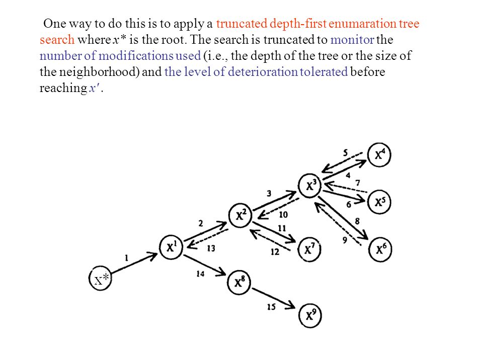
125. Exchange Procedure (EP) Variant of (VNS) with 2 neighborhood structures where the descent method (D) is the (LSM) used: i) Apply the descent method with neighborhood structure N(x) ii) Once a local minimum x* is reached, apply the descent method using an enlarged and more complex neighborhood EN(x) to find a new solution x' such that f(x') < f(x*). One way to do this is to apply a truncated depth-first enumaration tree search where x* is the root. The search is truncated to monitor the number of modifications used (i.e., the depth of the tree or the size of the neighborhood) and the level of deterioration tolerated before reaching x'.

127. Material from the following reference Jacques A. Ferland and Daniel Costa, “ Heuristic Search Methods for Combinatorial Programming Problems”, Publication # 1193, Dep. I. R. O., Université de Montréal, Montréal, Canada (March 2001)