1. Rotational Ambiguity in Soft- Modeling Methods

2. D = USV = u 1 s 11 v 1 + … + u r s rr v r Singular Value Decomposition Row vectors: d 1,: d 2,: d p,: … = u 11 u 21 u p1 … s 11 v1v1 u 12 u 22 u p2 … s 22 v2v2 + d 1,: = u 11 s 11 v 1 + u 12 s 22 v 2 d 2,: = …… d p,: = u 21 s 11 v 1 + u 22 s 22 v 2 u p1 s 11 v 1 + u p2 s 22 v 2 … For r=2 D = u 1 s 11 v 1 + u 2 s 22 v 2

3. D = USV = u 1 s 11 v 1 + … + u r s rr v r Singular Value Decomposition [ d :,1 d :,2 … d :,q ] = u 1 s 11 [v 11 v 12 … v 1q ] + u 1 s 22 [v 21 v 22 … v 2q ] d :,1 = s 11 v 11 u 1 + s 22 v 21 u 2 …… d :,2 = d :,q = s 11 v 12 u 1 + s 22 v 22 u 2 s 11 v 1q u 1 + s 22 v 2q u 2 For r=2 D = u 1 s 11 v 1 + u 2 s 22 v 2 Column vectors:

4. Rows of measured data matrix in row space: u 11 s 11 d 1,: v1v1 v2v2 u 12 s 22 d 2,: d p,: u 21 s 11 u 22 s 22 u p2 s 22 u p1 s 11 … u 11 s 11 u 12 s 22 … u 21 s 11 u 22 s 22 u p1 s 11 u p2 s 22 … Coordinates of rows

5. Columns of measured data matrix in column space: u1u1 u2u2 d :, 2 d :, 1 d :, q … v 2q s 22 v 1q s 11 v 12 s 11 v 22 s 22 v 21 s 22 v 11 s 11 v 11 s 11 v 12 s 11... v 1q s 11 Coordinates of columns v 21 s 11 v 22 s 11... v 2q s 11

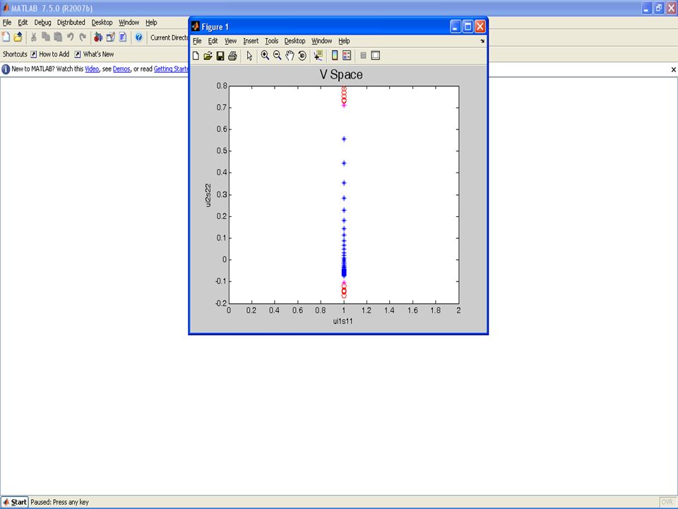
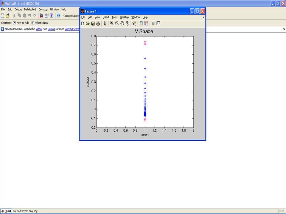
7. Visualizing the rows of data in V-space

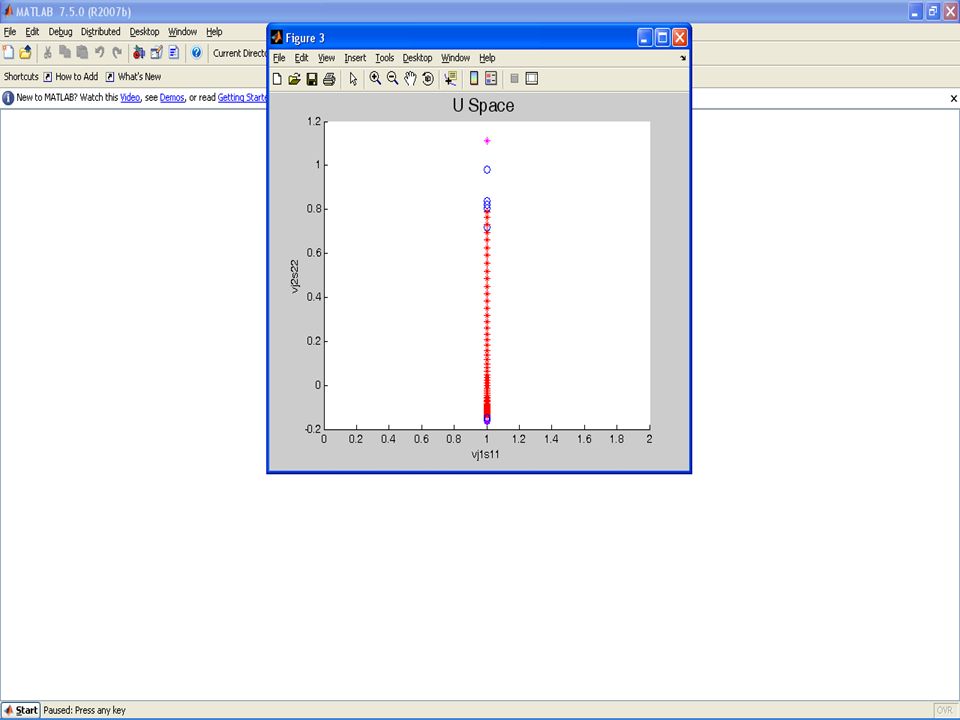
8. Visualizing the Columns of data in U-space

9. ScorePlot.m Visualizing the Rows and Columns of the Data

10. ? Investigate the effects of pure profiles overlapping on structure of measured data matrix using ScorePlot.m file

11. Solution of a soft-modeling method D = USV = CA C ≠ USA ≠ V D = US (T -1 T) V = CA C = US T -1 A =T V t 11 t 12 t 21 t 22 T= ti 11 ti 12 ti 21 ti 22 T -1 = Two component systems:

12. a 1 = t 11 v 1 + t 12 v 2 a 2 = t 21 v 1 + t 22 v 2 A = C = [c 1 = ti 11 s 11 u 1 + ti 21 s 22 u 2 c 2 = ti 12 s 11 u 1 + ti 22 s 22 u 2 ] Solution of a soft-modeling method The elements of T matrix are the coordinates of real spectral profiles in V space The elements of ST -1 matrix are the coordinates of real concentration profiles in U space

13. Rotational ambiguity The one major problem with all model-free methods is the fact that often there is no unique solution for the task of decomposing the data matrix into the product of two physically meaningful matrices. Where there is rotational ambiguity, the solution of soft-modeling methods is one particular point within the range of possibilities.

14. Intensity ambiguity in V space v1v1 v2v2 a k1ak1a k2ak2a T 11 T 12 k 1 T 11 k 1 T 12 k 2 T 11 k 2 T 12

15. Normalization a = T 1 v 1 + T 2 v 2 k 1 a = k 1 T 1 v 1 + k 1 T 2 v 2 k 2 a = k 2 T 1 v 1 + k 2 T 2 v 2 k n a = k n T 1 v 1 + k n T 2 v 2 … a’ = v 1 + T v 2

16. v1v1 v2v2 Normalization 1 1 2 4 3 5 a = T 1 v 1 + T 2 v 2 a’ = v 1 + T v 2 1’2’3’ 4’ 5’

17. n_V_U_space.m Visualizing the Normalized Data in Row and Column Space

47. Calculation and Visualization of Rotational Ambiguity D = C A + E = D * + E C new = C T A new = T -1 A D * = C A = (C T)(T -1 A) = C new A new Both solutions are equivalent: they have equal fit T is any invertible matrix and defines rotation ambiguities Only those T values fulfilling the constraints are considered feasible Bilinear model

48. MCR bilinear model PCA bilinear model For the simplest case of two components Normalization of the diagonal elements to one D = C A + R D = U V + R’ If R ≈ R’ A ≈ T V C ≈ T -1 U 1T 12 T 21 1 T = 1 - T 12 T 21 1-T 12 -T 21 1 1 T -1 = T 11 T 12 T 21 T 22 T = Calculation and Visualization of Rotational Ambiguity

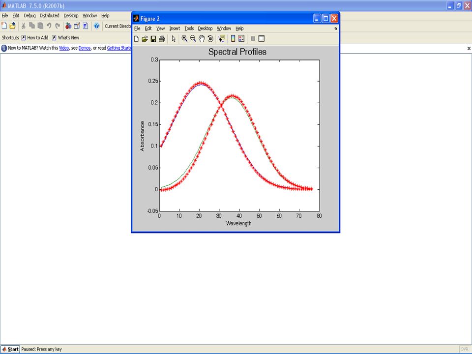
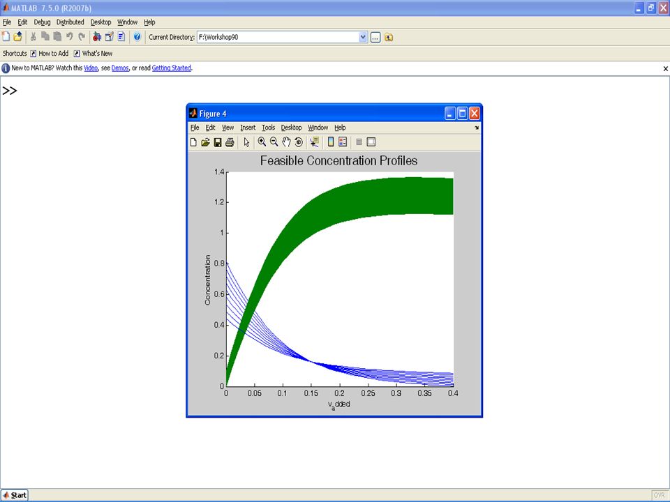
49. How the boundaries for a 1 and a 2 can be calculated? Calculation of A profiles as a function of (T 12,T 21 ) Shape and boundaries of a 1 and a 2 (and their norms) are defined respectively by T 12 and T 21 TV = 1T 12 T 21 1 v1v2v1v2 v 1 + T 12 v 2 T 21 v 1 + v 2 = A a1a2a1a2 = a 1 = v 1 + T 12 v 2 a 2 = T 21 v 1 + v 2 Calculation and Visualization of Rotational Ambiguity

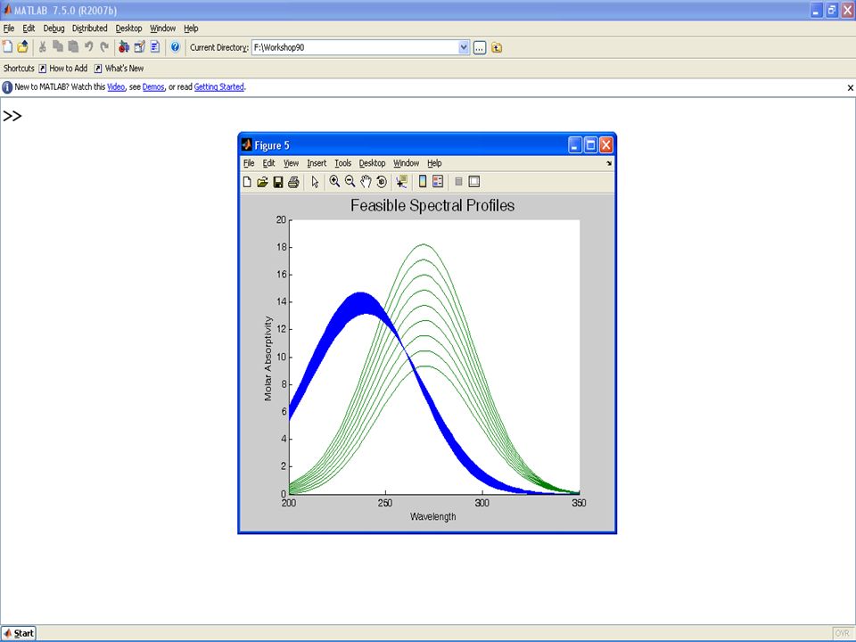
50. Calculation of C profiles as a function of (T 12,T 21 ) 1 - T 12 T 21 1-T 12 -T 21 1 1 UT -1 = [ u 1 u 2 ] = [ c 1 c 2 ]= C How the boundaries for a 1 and a 2 can be calculated? c 1 = (u 1 - T 21 u 2 ) 1 - T 12 T 21 1 c 2 = (-T 12 u 1 + u 2 ) 1 - T 12 T 21 1 Shape and boundaries of c 1 and c 2 (and their norms) are defined respectively by T 12, T 21 and eigenvalues of DD T Calculation and Visualization of Rotational Ambiguity

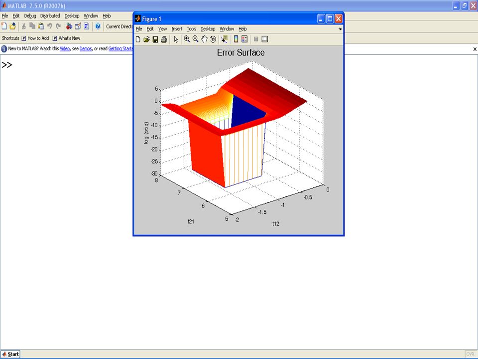
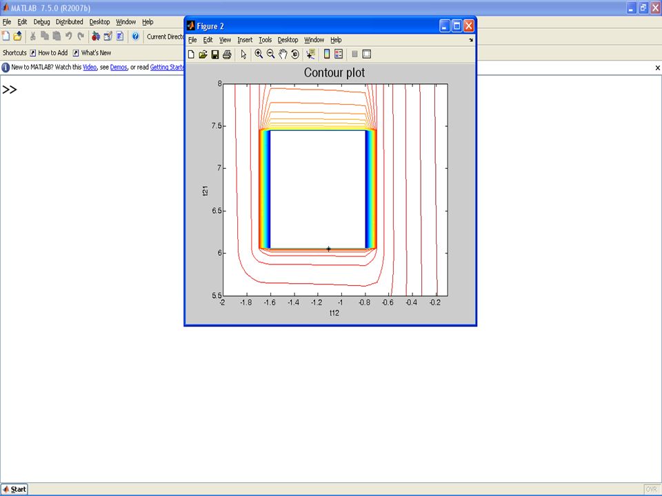
51. Rotational ambiguity region: Solutions fitting equally well the data and fulfilling the constraints of the system ssq =  ( D - CA) 2 =  (r ij 2 ) = f (T 12, T 21 ) Look for min log(ssq) under non-negativity constraints using a grid search residuals minimization Calculation and Visualization of Rotational Ambiguity

52. GridSearch2.m Calculation of Feasible Solutions in 2 Components System

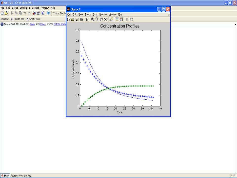
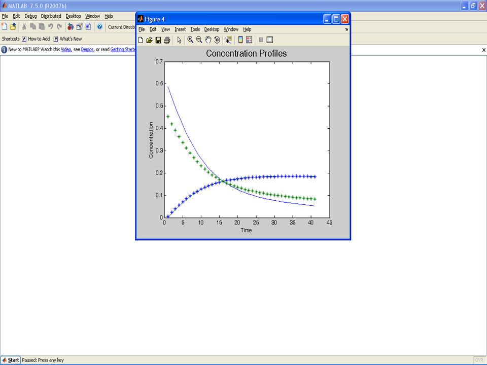
58. ? Investigate the effects of overlapping and noise on feasible solutions

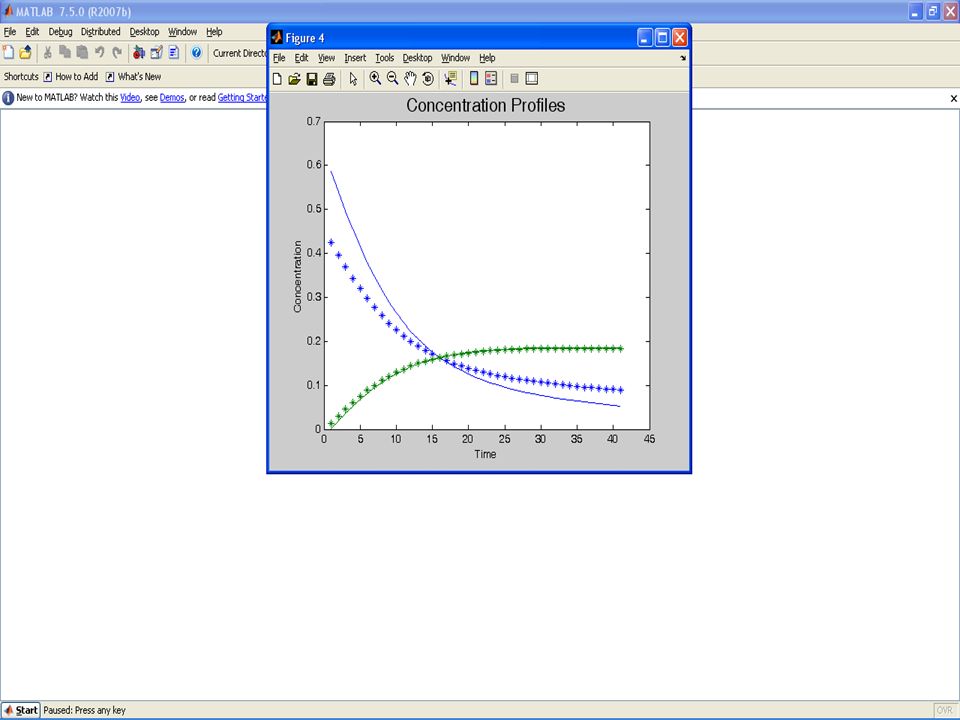
59. Main_Conc.m Uncertainty in Soft- Modeling then Fitting

61. ? Fit the concentration profile of each component individually