1. RELIABILITY DESIGN of TRANSPORTATION NETWORK: ANALYSIS and PREDISASTER MANAGEMENT I. GERTSBAKH and Y. SHPUNGIN ניהול תרום-משברי של רשת דרכים BGU, MATHEMATICS DEPARTMENT SAMI SHAMOON COLLEGE OF ENGINEERING, COMPUTER SCIENCE DEPARTMENT, BEER-SHEVA

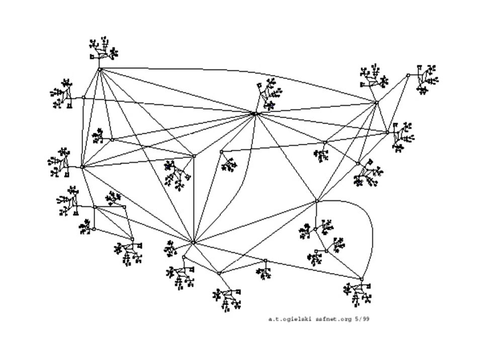
7. NODE LINK TERMINAL NODE Important: It can be a communication network, water, oil or food supply network, etc

8. 11109816715614541332121 18 Intersection, hospital, storage, city Roads, bridges, tunnels, supply channels, water pipes,etc TERMINAL Network 17

9. 111017 9816715614541332 121 18 LINK FAILURE DISASTER: earthquake, disruption, damage, accident, enemy attack Terminal Connectivity may be disrupted when links fail randomly

10. P P P* 0.5 0.9 COST: C reinforcement

11. IMPORTANT: TO UNDERSTAND WHAT MEANS “PROBABILITY OF TERMINAL CONNECTIVITY” 1 23 All nodes are terminals LET EDGE BE OPERATiING WITH PROBABILITY P=0.5 PROBABILITY OF TERMINAL CONNECTIVITY = 0.5 SUPPOSSUPPOS SUPPOSE THAT WE REINFORCE EACH LINK AND NOW LINK RELIABILITY WILL BE 0.7. THEN ALL-NODE RELIABILITY WILL BE 0.784

12. SUPPOSE ONLY TWO NODES ARE TERMINALS: HERE THE PROBABILIY OF TWO-TERMINAL CONNECTIVITY IS 0.625 NOW SUPPOSE THAT WE REINFORCE EACH LINK AND THE PROBABILITY THAT IT IS OPERATING EQUALS NOW 0.7 (BEFORE IT WAS O.5) NOW THE PROBABILITY OF TWO-TERMINAL CONNECTIVITY WILL BE 0.820

13. The GOAL FUNCTION (CRITERION) : MAXIMIZE the PROBABILITY of SAFE CONNECTION BETWEEN The TERMINALS By the BEST choice of the links which have to be REINFORCED And subject to the BUDGET CONSTRAINTS OR: reach the desired level of reliability R* for minimal cost

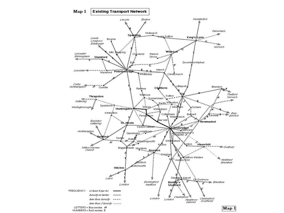
15. 1 3 4 2 5 8 10 6 7 9 24 11 25 12 13 14 15 20 19 22 23 18 21 17 16 1 3 2 2 4 5 7 6 12 9 8 10 13 11 15 16 14 19 18 17 20 21 22 25 27 28 30 29 26 24 Important connections: (14,20), (14,7), (12,18), (9,7), (4,8) 30-link network of ISTANBUL, 25 nodes TURKEY 23

16. Parameters of the Problem: Link failure – due to earthquake Each link has its failure probability ranging from 0.2 to 0.5 Link j reinforcement costs c(j) Reinforcement of any link reduces its failure probability to ZERO The GOAL : to MAXIMIZE the PROBABILITY of SAFE CONNECTION BETWEEN THE FIVE PAIRS OF NODES The total cost of reinforcement should NOT exceed the given budget B INDEPENDENT link failures (not realistic !) 80-1200 B<= 1700

17. The source: Pre-disaster investment decisions for strengthening a highway network 2010, S. Pieta, Sibel Salman, D.Gunnec, K Viswatath,..

18. THE SOLUTION ALGORITHM ( Salman, Pieta) Not simple one! 10, 20, 21, 22, 23, 25 The Cost=1640 THE AVERAGE RELIABILITY is about 0.80 The MINIMAL reliability of a single pair (14,7) and (4,8) is 0.672 Solution procedure Reinforce links: DATA

20. 1 3 4 2 5 8 10 6 7 9 24 11 25 12 13 14 15 20 19 22 23 18 21 17 16 1 3 2 2 4 5 7 6 12 9 8 10 13 11 15 16 14 19 18 17 20 21 22 25 27 28 30 29 26 24 Important connections: (14,20), (14,7), (12,18), (9,7), (4,8) 30-link network of ISTANBUL, 25 nodes TURKEY 23

21. KNAPSACK ALGORITHM Our solution: our Objective: maximize the MINIMAL CONNECTION PROBABILITY IN the FIVE PAIRS FOR EACH REINFORCED LINK CONSIDER THE minCONNECTION PROBABILITY INCREASE PER UNIT OF COST : PROBABILITY INCREASE/COST REINFORCE THAT LINK WHICH MAXIMIZES THIS RATIO Proceed within the BUDGET

22. OUR RESULTS : REINFORCE LINKS :10, 17, 20, 21, 22, 23 OUR COST IS 1700 The MINIMAL CONNECTION PROBBILITYY is 0.682 THE AVERAGE CONNECTION PROBABILITY is 0.803 ALMOST IDENTICAL TO Salman- Pieta SOLUTION

23. The Principle of Incompatibility. The principle states that as a system complexity increases, our ability to make absolute, precise and significant statements about the system’s behavior diminishes until a threshold, fuzzily defined, is reached. Beyond that threshold precision and significance are mutually exclusive. For this reason… precise quantitative analysis and high complexity in incompatible with absolute precision. Management is always a venture of reducing or compressing complex realities. The full implication of this principle is not realized until a corollary principle is managed: THE CLOSER ONE LOOKS AT A REAL WORLD PROBLEM, THE FUZZIER ITS SOLUTIONS. L.Zadeh

24. OUR NETWORK : 25 nodes, 34 links, 4 terminals 1 23 21 17 18 3 2 4 5 8 9 10 7 22 20 19 16 14 15 12 13 11 6 24 25 min cuts of size 3 13 p=0.7 => R=0.476 - very low !!

25. SCENARIO A: ALL p=0.7, REINFORCED TO P*=0.9;EQUAL 1 23 21 17 18 3 2 4 5 8 9 10 7 22 20 19 16 14 15 12 13 11 6 24 25 min cuts of size 3 13 p=0.7 => 0.9R*=0.842 COSTS Reinforced Shown BOLD

26. SCENARIO B: p=0.6, 0.7,0.8; P*=0.9; ALL COSTS ARE C=1 1 23 21 17 18 3 2 4 5 8 9 10 7 22 20 19 16 14 15 12 13 11 6 24 25 -

27. Initial Reliability of connectivity=0.471 Edges for reinforcement are chosen by the largest values of Derivative x (0.9- p) Edges chosen are : (1,3), (3,5),(7,11) (9,11),(12,13),(12,16),(13,14),(15,24), (216,17),(18,20),(18,21),(19,25): Reinforcement costs are = 1

28. SOLUTION PROCEDURE: The main problem is finding the GRADIENT vector

29. SCENARIO B: p=0.6, 0.7,0.8; P*=0.9; ALL COSTS ARE C=1 1 23 21 17 18 3 2 4 5 8 9 10 7 22 20 19 16 14 15 12 13 11 6 24 25 - Initial R=0.471 R*=0.85

30. SCENARIO C: p=0.6, 0.7,0.8; P*=0.9; COSTS ARE C=1,2,3,4 1 23 21 17 18 3 2 4 5 8 9 10 7 22 20 19 16 14 15 12 13 11 6 24 25 - 2 3 4 2 3 4 2 3 4 2 3 4 2 3 4 2 3 4 2 3 4 2 3 4 2 1 1 1 1 1 1 1

31. The total cost in scenario B was 30 In scenario C we compute for each link the ratio: Gradient of the link x (0.9-p) Link cost Take maximal SOLUTION: REINFORCE THE LINKS (7,11), (15,24), (18,21), (3,5),(12,13),(21,23), (1,2),(5,10),(9,24),(11,13), (1,3), (13,14) R*=0.848TOTAL COST =20 If we take 12 edges with min Cost R=0.684 total cost=12 Knapsack approach

32. SCENARIO C: p=0.6, 0.7,0.8; P*=0.9; COSTS ARE C=1,2,3,4 1 23 21 17 18 3 2 4 5 8 9 10 7 22 20 19 16 14 15 12 13 11 6 24 25 - 2 3 4 2 3 4 2 3 4 2 3 4 2 3 4 2 3 4 2 3 4 2 3 4 2 1 1 1 1 1 1 1 1 1 1

33. SOLUTION PROCEDURE: The main problem is finding the GRADIENT vector

34. s t 1 9 1 1 8 1 8 1 8 1 2 6 7 5 3 4 7, 3, 5, 4, 8, 9, 2, 1, 6 s t DOWN states The UP state The BORDER state Activated by edge 9

35. s t 8 7 5 3 4 RULE: Partial Derivative of R w.r. to p(9)=[ The probability of all border states “activated” by edge 9]/q(9) 9

36. Algorithm: Simulate a permutation of edge numbers Create the corresponding evolution process and identify the border state and the last “activating” edge For each edge, find out all border states “activated” by this edge and compute their probability Repeat M times

37. SOLUTION PROCEDURE: The main problem is finding the GRADIENT vector

38. References: Pre-disaster investment decisions for strengthening a highway network 2010, S. Pieta, Sibel Salman, D.Gunnec, K Viswatath A transport network reliability model for the efficient assignment of resources, 2005, M. Sanchez-Silva et al. 1.. Optimal Reliability design of transportation network, 2010, Gertsbakh, Shpungin, RelStat10, Conference, Riga. 5 Models of Network Reliability: Analysis, Combinatorics, and Monte Carlo CRC Press, 2009, I.Gertsbakh and Y. Shpungin 212212 Predisaster Design of Transportation Network, 2011,Transport and Telecommunication Scientific & Research Journal of TTI, Vol12, No 1,, 4-11., Shpungin Y. and I. Gertsbakh.

39. References: Pre-disaster investment decisions for strengthening a highway network 2010, S. Pieta, Sibel Salman, D.Gunnec, K Viswatath,..

40. Thank you for Attention