1. Discriminative Frequent Pattern Analysis for Effective Classification By Hong Cheng, Xifeng Yan, Jiawei Han, Chih- Wei Hsu Presented by Mary Biddle

2. Introduction Pattern Example Patterns –ABCD –ABCF –BCD –BCEF Frequency –A = 2 –B = 4 –C = 4 –D = 2 –E = 1 –F = 2 –AB = 2 –BC = 4 –CD = 2 –CE = 1 –CF = 2

3. Motivation Why are frequent patterns useful for classification? Why do frequent patterns provide a good substitute for the complete pattern set? How does frequent pattern-based classification achieve both high scalability and accuracy for the classification of large datasets? What is the strategy for setting the minimum support threshold? Given a set of frequent patterns, how should we select high quality ones for effective classification?

4. Information Fisher Score Definition In statistics and information theory, the Fisher Information is the variance of the score. The Fisher information is a way of measuring the amount of information that an observable random variable X carries about an unknown parameter θ upon which the likelihood function of θ, L(θ) = f(X, θ), depends. The likelihood function is the joint probability of the data, the Xs, conditional on the value of θ, as a function of θ.

5. Introduction Information Gain Definition In probability theory and information theory Information Gain is a measure of the difference between two probability distributions: from a “true” probability distribution P to an arbitrary probability distribution Q. The expected Information Gain is the change in information entropy from a prior state to a state that take some information as given. Usually an attribute with high information gain should be preferred to other attributes.

6. Model Combined Feature Definition Each (attribute, value) pair is mapped to a distinct item in I = {o 1,…,o d }. A combined feature α = {o α1,…,o αk } is a subset of I, where o α i {o 1,…,o d }, 1 ≤ i ≤ k o i I is a single feature. Given a dataset D = {x i }, the set of data that contains α is denoted as D α = {x i |x iα j = 1, o α j α}.

7. Model Frequent Combined Feature Definition For a dataset D, a combined feature α is frequent if θ = |D α |/|D| ≥ θ 0, where θ is the relative support of α, and θ 0 is the min_sup threshold, 0 ≤ θ 0 ≤ 1. The set of frequent defined features is denoted as F.

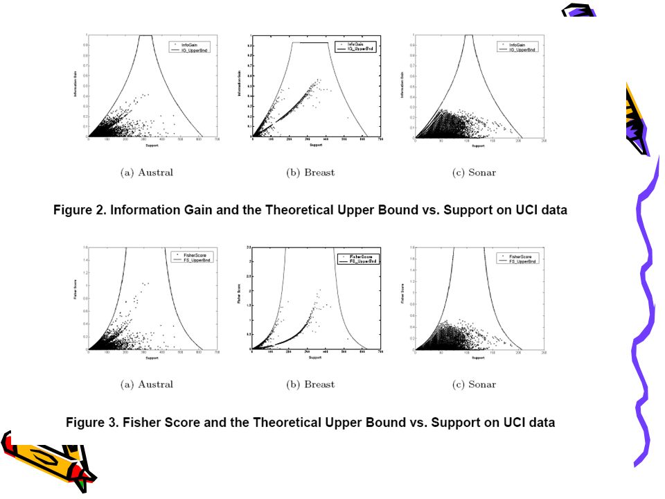
8. Model Information Gain For a patter α represented by a random variable X, the information gain is IG(C|X) = H(C)-H(C|X) Where H(C) is the entropy And H(C|X) is the conditional entropy Given a dataset with a fixed class distribution, H(C) is a constant.

9. Model Information Gain Upper Bound The information gain upper bound IG ub is IG ub (C|X) = H(C) - H lb (C|X) Where H lb is the lower bound of H(C|X)

10. Model Fisher Score Fisher score is defined as Fr = (∑ c i=1 n i (u u i -u) 2 )/ (∑ c i=1 n i σ i 2 ) where n i is the number of data samples in class i, u u i is the average feature value in class i σ i is the standard deviation of the feature value in class i u is the average feature value in the whole dataset.

12. Model Relevance Measure S A relevance measure S is a function mapping a pattern α to a real value such that S(α) is the relevance w.r.t. the class label. Measures like information gain and fisher score can be used as a relevance measure.

13. Model Redundancy Measure A redundancy measure R is a function mapping two patterns α and ß to a real value such that R(α, ß) is the redundancy between them. R(α, ß) = (P(α, ß) / (P(α) + P(ß) – P(α,ß) ))x min(S(α),S(ß)) P is the predicate function from the Jaccard measure.

14. Model information gain The gain of a pattern α given a set of already selected patterns F s is g(α)=S(α)-maxR(α, ß) Where ß F s

15. Algorithm framework of frequent pattern-based classification 1.Feature generation 2.Feature selection 3.Model learning

16. Algorithm 1. Feature Generation 1.Compute information gain (or Fisher score) upper bound as a function of support θ. 2.Choose an information gain threshold IG 0 for feature filtering purposes. 3.Find θ* = arg max θ (IG ub (θ)≤IG 0 ) 4.Mine frequent patterns with min_sup = θ*

17. Algorithm 2. Feature Selection Algorithm MMRFS

18. Algorithm 3. Model Learning Use the resulting features as input to the learning model of your choice. –They experimented with SVM and C4.5

19. Contributions Propose a framework of frequent pattern-based classification by analyzing the relationship between pattern frequency and its predictive power. Frequent pattern-based classification could exploit the state-of-the-art frequent pattern mining algorithms for feature generation with much better scalability. Suggest a strategy for setting a minimum support. An effective and efficient feature selection algorithm is proposed to select a set of frequent and discriminative patterns for classification.

20. Experiments Accuracy with SVN and C4.5

21. Experiments Accuracy and Time Measures

22. Related Work Associative Classification –The association between frequent patterns and class labels is used for prediction. A classifier is built based on high-confidence, high-support association rules. Top-K rule mining –A recent work on top-k rule mining discovers top-k covering rule groups for each row of gene expression profiles. Prediction is perfomed based on a classification score which combines the support and confidence measures of the rules. HARMONY (mines classification rules) –It uses an instance-centric rule-generation approach and assures for each training instance, that one of the highest confidence rules covering the instance is included in the rule set. This is the more efficient and scalable than previous rule-based classifiers. On several datasets the classifier accuracy was significantly higher, i.e. 11.94% on Waveform and 3.4% on Letter Recognition. All of the following use frequent patterns –String kernels –Word combinations (NLP) –Structural features in graph classification

23. Differences between Associative Classification and Discriminative Frequent Pattern Analysis Classification Frequent Patterns are used to represent the data in a different feature space. Associative classification builds a classification using rules only. In associative classification, the prediction process is to find one or several top ranked rule(s) for prediction. In this process, the prediction is made by the classification model. The information gain is used to discriminate the patterns being used by using it to determine the min_sup and in the selection of the frequent patterns.

24. Pros and Cons Pros –Reduces Time –More accurate Cons –Space concerns on large datasets because it uses the entire Pattern set, initially.