Download presentation
Presentation is loading. Please wait.

1
Chapter 6 Graphs

2
2 Outline Definitions, Terminologies and Applications Graph Representation Elementary graph operations Famous Graph Problems

3
3 Graphs G = (V,E) V is the vertex set. Vertices are also called nodes and points. E is the edge set. Each edge connects two different vertices. Undirected edge has no orientation (u,v). Directed edge has an orientation (u,v). uv uv
. Directed edge has an orientation (u,v). uv uv.")
4
4 Graph Undirected graph => no oriented edge Directed graph => every edge has an orientation Proper graph No loops No multi-edges

5
5 Undirected Graph 2 3 8 10 1 4 5 9 11 6 7

6
6 Directed Graph (Digraph) 2 3 8 10 1 4 5 9 11 6 7
")
7
7 Examples of Graphlike Structures 0 2 1 1 2 3 0 (a) Graph with a self edge (b) Multigraph
 Graph with a self edge (b) Multigraph")
8
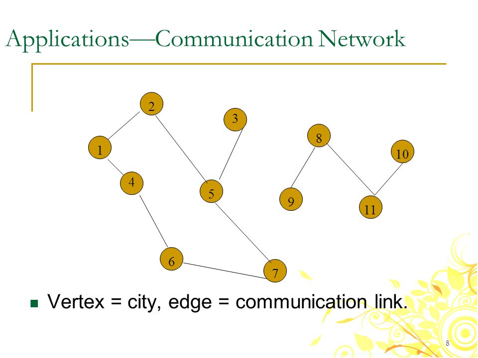
8 Applications — Communication Network Vertex = city, edge = communication link. 2 3 8 10 1 4 5 9 11 6 7
9
9 Driving Distance/Time Map Vertex = city, edge weight = driving distance/time. Weighted undirected graph 2 3 8 10 1 4 5 9 11 6 7 4 8 6 6 7 5 2 4 4 5 3

10
10 Street Map Some streets are one way. 2 3 8 10 1 4 5 9 11 6 7

11
Terminologies Vertex, edge, directed, undirected, weighted, unweighted Adjacenct Subgraph Path A path from u to v in graph G is a sequence of vertices u,i 1, i 2,…,j k, v such that (u, i 1 )…(i k, v) are edges in E(G). The length of a path is the number of edges on it. Simple path All vertices except possibly the first and last are distinct Cycle A simple path whose first and last vertices are the same

12
12 G 1 and G 3 Subgraphs 0 3 12 0 3 12 0 12 0 0 1 2 0 1 2 0 1 2 (a) Some subgraphs of G 1 (a) Some subgraphs of G 3 (i) (ii) (iii) (iv) (i) (ii) (iii) (iv)
 Some subgraphs of G 1 (a) Some subgraphs of G 3 (i) (ii) (iii) (iv) (i) (ii) (iii) (iv)")
13
13 Terminologies Undirected graph Connected Vertices Graph Connected component Maximal connected subgraph degree

14
14 Terminologies Directed graph Strongly connected Strongly connected component A maximal subgraph that is strongly connected indegree outdegree Acyclic Cycle free graph

15
15 Complete Undirected Graph Has all possible edges. n = 1 n = 2 n = 3 n = 4

16
16 Number Of Edges — Undirected Graph Each edge is of the form (u,v), u != v. Number of such pairs in an n vertex graph is n(n-1). Since edge (u,v) is the same as edge (v,u), the number of edges in a complete undirected graph is n(n-1)/2. Number of edges in an undirected graph is <= n(n-1)/2.
. Since edge (u,v) is the same as edge (v,u), the number of edges in a complete undirected graph is n(n-1)/2. Number of edges in an undirected graph is <= n(n-1)/2..")
17
17 Number Of Edges — Directed Graph Each edge is of the form (u,v), u != v. Number of such pairs in an n vertex graph is n(n-1). Since edge (u,v) is not the same as edge (v,u), the number of edges in a complete directed graph is n(n-1). Number of edges in a directed graph is <= n(n-1).
. Since edge (u,v) is not the same as edge (v,u), the number of edges in a complete directed graph is n(n-1). Number of edges in a directed graph is <= n(n-1)..")
18
18 Sum Of Vertex Degrees Sum of degrees = 2e (e is number of edges) 8 10 9 11
")
19
19 Sum Of In- And Out-Degrees each edge contributes 1 to the in-degree of some vertex and 1 to the out-degree of some other vertex sum of in-degrees = sum of out-degrees = e, where e is the number of edges in the digraph

20
20 Graph Representation Adjacency Matrix Adjacency Lists

21
21 Adjacency Matrix 0/1 n x n matrix, where n = # of vertices A(i,j) = 1 iff (i,j) is an edge 2 3 1 4 5 12345 1 2 3 4 5 01010 10001 00001 10001 01110
 = 1 iff (i,j) is an edge")
22
22 Adjacency Matrix Properties 2 3 1 4 5 12345 1 2 3 4 5 01010 10001 00001 10001 01110 Diagonal entries are zero. Adjacency matrix of an undirected graph is symmetric. A(i,j) = A(j,i) for all i and j.
 = A(j,i) for all i and j..")
23
23 Adjacency Matrix (Digraph) 2 3 1 4 5 12345 1 2 3 4 5 00010 10001 00000 00001 01100 Diagonal entries are zero. Adjacency matrix of a digraph need not be symmetric.

24
24 Adjacency Matrix n 2 bits of space For an undirected graph, may store only lower or upper triangle (exclude diagonal). (n-1)n/2 bits O(n) time to find vertex degree and/or vertices adjacent to a given vertex.
n/2 bits O(n) time to find vertex degree and/or vertices adjacent to a given vertex..")
25
25 Adjacency Lists Adjacency list for vertex i is a linear list of vertices adjacent from vertex i. An array of n adjacency lists. 2 3 1 4 5 aList[1] = (2,4) aList[2] = (1,5) aList[3] = (5) aList[4] = (5,1) aList[5] = (2,4,3)
 aList[2] = (1,5) aList[3] = (5) aList[4] = (5,1) aList[5] = (2,4,3).")
26
26 Linked Adjacency Lists Each adjacency list is a chain. 2 3 1 4 5 aList[1] aList[5] [2] [3] [4] 24 15 5 51 243 Array Length = n # of chain nodes = 2e (undirected graph) # of chain nodes = e (digraph)
 # of chain nodes = e (digraph).")
27
27 Weighted Graphs Cost adjacency matrix. C(i,j) = cost of edge (i,j) Adjacency lists => each list element is a pair (adjacent vertex, edge weight)
 = cost of edge (i,j) Adjacency lists => each list element is a pair (adjacent vertex, edge weight).")
28
28 Elementary graph operations Visit a Graph (graph search) Connected components Spanning trees Biconnected components
 Connected components Spanning trees Biconnected components")
29
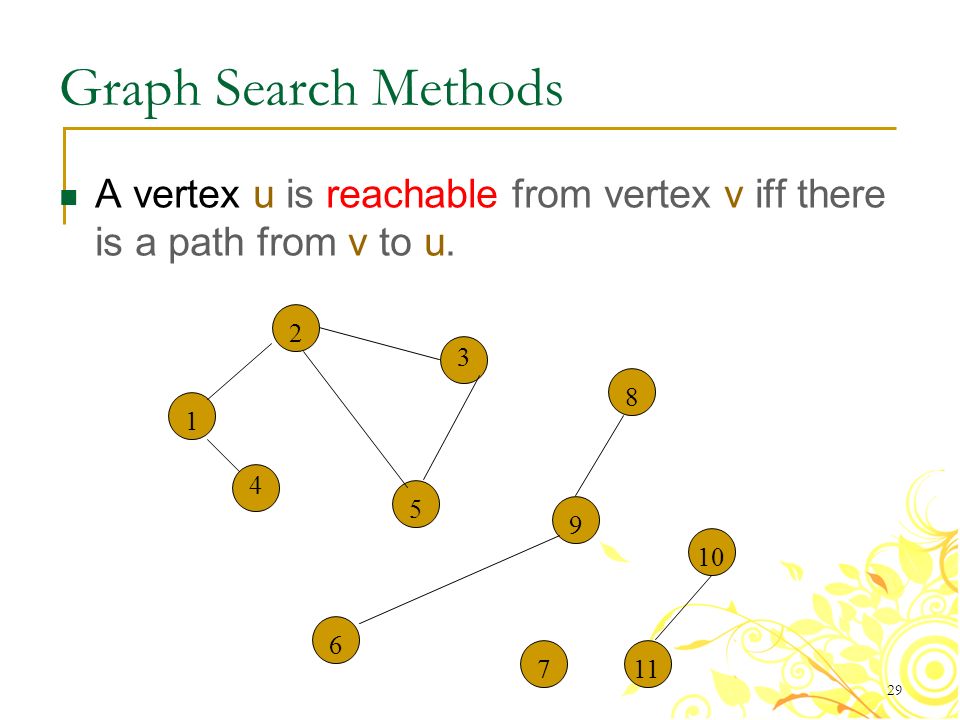
29 Graph Search Methods A vertex u is reachable from vertex v iff there is a path from v to u. 2 3 8 10 1 4 5 9 11 6 7
30
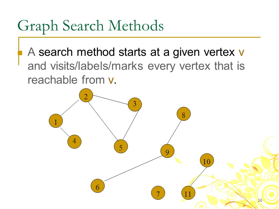
30 Graph Search Methods A search method starts at a given vertex v and visits/labels/marks every vertex that is reachable from v. 2 3 8 10 1 4 5 9 11 6 7
31
31 Graph Search Methods Many graph problems solved using a search method. Path from one vertex to another. Is the graph connected? Find a spanning tree. Etc. Commonly used search methods: Depth-first search. Breadth-first search.

32
32 Depth-First Search Example Start search at vertex 1. 2 3 8 10 1 4 5 9 11 6 7 Label vertex 1 and do a depth first search from either 2 or 4. 12 Suppose that vertex 2 is selected.

33
33 Depth-First Search Example 2 3 8 10 1 4 5 9 11 6 7 Label vertex 2 and do a depth first search from either 3, 5, or 6. 1225 Suppose that vertex 5 is selected.

34
34 Depth-First Search Example 2 3 8 10 1 4 5 9 11 6 7 Label vertex 5 and do a depth first search from either 3, 7, or 9. 122559 Suppose that vertex 9 is selected.

35
35 Depth-First Search Example 2 3 8 10 1 4 5 9 11 6 7 Label vertex 9 and do a depth first search from either 6 or 8. 12255998 Suppose that vertex 8 is selected.

36
36 Depth-First Search Example 2 3 8 10 1 4 5 9 11 6 7 Label vertex 8 and return to vertex 9. 122559988 From vertex 9 do a DFS(6). 6
. 6.")
37
37 Depth-First Search Example 2 3 8 10 1 4 5 9 11 6 7 122559988 Label vertex 6 and do a depth first search from either 4 or 7. 66 4 Suppose that vertex 4 is selected.

38
38 Depth-First Search Example 2 3 8 10 1 4 5 9 11 6 7 122559988 Label vertex 4 and return to 6. 66 44 From vertex 6 do a DFS(7). 7
. 7.")
39
39 Depth-First Search Example 2 3 8 10 1 4 5 9 11 6 7 122559988 Label vertex 7 and return to 6. 66 44 77 Return to 9.

40
40 Depth-First Search Example 2 3 8 10 1 4 5 9 11 6 7 12255998866 44 77 Return to 5.

41
41 Depth-First Search Example 2 3 8 10 1 4 5 9 11 6 7 12255998866 44 77 Do a DFS(3). 3
. 3")
42
42 Depth-First Search Example 2 3 8 10 1 4 5 9 11 6 7 12255998866 44 77 Label 3 and return to 5. 33 Return to 2.

43
43 Depth-First Search Example 2 3 8 10 1 4 5 9 11 6 7 12255998866 44 77 33 Return to 1.

44
44 Depth-First Search Example 2 3 8 10 1 4 5 9 11 6 7 12255998866 44 77 33 Return to invoking method.

45
45 Depth-First Search DFS() { for (i=0 to n-1) visited[i]=0; for (v=0 to n-1) { if (visted[v]==0) DFV(v); } DFV(v) { visited[v]=1; //Label vertex v as visited. for ( each unvisited vertex u adjacent from v ) DFV(u); }
![45 Depth-First Search DFS() { for (i=0 to n-1) visited[i]=0; for (v=0 to n-1) { if (visted[v]==0) DFV(v); } DFV(v) { visited[v]=1; //Label vertex v as visited.](http://images.slideplayer.com/28/9329314/slides/slide_45.jpg "for ( each unvisited vertex u adjacent from v ) DFV(u); }.")
46
46 Depth-First Search Property All vertices reachable from the start vertex (including the start vertex) are visited. Time complexity O(n 2 ) when adjacency matrix used O(n+e) when adjacency lists used (e is number of edges)
 when adjacency matrix used O(n+e) when adjacency lists used (e is number of edges).")
47
47 Breadth-First Search Visit start vertex and put into a FIFO queue. Repeatedly remove a vertex from the queue, visit its unvisited adjacent vertices, put newly visited vertices into the queue.

48
48 Breadth-First Search Example Start search at vertex 1. 2 3 8 10 1 4 5 9 11 6 7

49
49 Breadth-First Search Example Visit/mark/label start vertex and put in a FIFO queue. 2 3 8 10 1 4 5 9 11 6 7 1 FIFO Queue 1

50
50 Breadth-First Search Example Remove 1 from Q; visit adjacent unvisited vertices; put in Q. 2 3 8 10 1 4 5 9 11 6 7 1 FIFO Queue 1

51
51 Breadth-First Search Example Remove 1 from Q; visit adjacent unvisited vertices; put in Q. 2 3 8 10 1 4 5 9 11 6 7 1 FIFO Queue 2 2 4 4

52
52 Breadth-First Search Example Remove 2 from Q; visit adjacent unvisited vertices; put in Q. 2 3 8 10 1 4 5 9 11 6 7 1 FIFO Queue 2 2 4 4

53
53 Breadth-First Search Example Remove 2 from Q; visit adjacent unvisited vertices; put in Q. 2 3 8 10 1 4 5 9 11 6 7 1 FIFO Queue 2 4 4 5 5 3 3 6 6

54
54 Breadth-First Search Example Remove 4 from Q; visit adjacent unvisited vertices; put in Q. 2 3 8 10 1 4 5 9 11 6 7 1 FIFO Queue 2 4 4 5 5 3 3 6 6

55
55 Breadth-First Search Example Remove 4 from Q; visit adjacent unvisited vertices; put in Q. 2 3 8 10 1 4 5 9 11 6 7 1 FIFO Queue 2 4 5 5 3 3 6 6

56
56 Breadth-First Search Example Remove 5 from Q; visit adjacent unvisited vertices; put in Q. 2 3 8 10 1 4 5 9 11 6 7 1 FIFO Queue 2 4 5 5 3 3 6 6

57
57 Breadth-First Search Example Remove 5 from Q; visit adjacent unvisited vertices; put in Q. 2 3 8 10 1 4 5 9 11 6 7 1 FIFO Queue 2 4 5 3 3 6 6 9 9 7 7

58
58 Breadth-First Search Example Remove 3 from Q; visit adjacent unvisited vertices; put in Q. 2 3 8 10 1 4 5 9 11 6 7 1 FIFO Queue 2 4 5 3 3 6 6 9 9 7 7

59
59 Breadth-First Search Example Remove 3 from Q; visit adjacent unvisited vertices; put in Q. 2 3 8 10 1 4 5 9 11 6 7 1 FIFO Queue 2 4 5 3 6 6 9 9 7 7

60
60 Breadth-First Search Example Remove 6 from Q; visit adjacent unvisited vertices; put in Q. 2 3 8 10 1 4 5 9 11 6 7 1 FIFO Queue 2 4 5 3 6 6 9 9 7 7

61
61 Breadth-First Search Example Remove 6 from Q; visit adjacent unvisited vertices; put in Q. 2 3 8 10 1 4 5 9 11 6 7 1 FIFO Queue 2 4 5 3 69 9 7 7

62
62 Breadth-First Search Example Remove 9 from Q; visit adjacent unvisited vertices; put in Q. 2 3 8 10 1 4 5 9 11 6 7 1 FIFO Queue 2 4 5 3 69 9 7 7

63
63 Breadth-First Search Example Remove 9 from Q; visit adjacent unvisited vertices; put in Q. 2 3 8 10 1 4 5 9 11 6 7 1 FIFO Queue 2 4 5 3 697 7 8 8

64
64 Breadth-First Search Example Remove 7 from Q; visit adjacent unvisited vertices; put in Q. 2 3 8 10 1 4 5 9 11 6 7 1 FIFO Queue 2 4 5 3 697 7 8 8

65
65 Breadth-First Search Example Remove 7 from Q; visit adjacent unvisited vertices; put in Q. 2 3 8 10 1 4 5 9 11 6 7 1 FIFO Queue 2 4 5 3 6978 8

66
66 Breadth-First Search Example Remove 8 from Q; visit adjacent unvisited vertices; put in Q. 2 3 8 10 1 4 5 9 11 6 7 1 FIFO Queue 2 4 5 3 6978 8

67
67 Breadth-First Search Example Queue is empty. Search terminates. 2 3 8 10 1 4 5 9 11 6 7 1 FIFO Queue 2 4 5 3 6978

68
BFS(int v) { for (i=0 to n-1) visited[i]=0; queue_insert(v); visited[v]=1; while (queue is not empty) { v=queue_delete(); for each unvisited vertex w adjacent to v { queue_insert(w); visited[w]=1; } 68
![BFS(int v) { for (i=0 to n-1) visited[i]=0; queue_insert(v); visited[v]=1; while (queue is not empty) { v=queue_delete(); for each unvisited vertex w adjacent to v { queue_insert(w); visited[w]=1; } 68](http://images.slideplayer.com/28/9329314/slides/slide_68.jpg "BFS(int v) { for (i=0 to n-1) visited[i]=0; queue_insert(v); visited[v]=1; while (queue is not empty) { v=queue_delete(); for each unvisited vertex w adjacent to v { queue_insert(w); visited[w]=1; } 68")
69
69 BFS() { for (i=0 to n-1) visited[i]=0; while (there is any unvisted node v) { queue_insert(v); visited[v]=1; while (queue is not empty) { v=queue_delete(); for each unvisited vertex w adjacent to v { queue_insert(w); visited[w]=1; }
![69 BFS() { for (i=0 to n-1) visited[i]=0; while (there is any unvisted node v) { queue_insert(v); visited[v]=1; while (queue is not empty) { v=queue_delete(); for each unvisited vertex w adjacent to v { queue_insert(w); visited[w]=1; }](http://images.slideplayer.com/28/9329314/slides/slide_69.jpg "69 BFS() { for (i=0 to n-1) visited[i]=0; while (there is any unvisted node v) { queue_insert(v); visited[v]=1; while (queue is not empty) { v=queue_delete(); for each unvisited vertex w adjacent to v { queue_insert(w); visited[w]=1; }")
70
70 Breadth-First Search Properties Same complexity as DFS. Time complexity O(n 2 ) when adjacency matrix used O(n+e) when adjacency lists used (e is number of edges)
 when adjacency matrix used O(n+e) when adjacency lists used (e is number of edges).")
71
71 Is The Graph Connected? Start a depth-first search at any vertex of the graph. Graph is connected iff all n vertices get visited. Time O(n 2 ) when adjacency matrix used O(n+e) when adjacency lists used (e is number of edges)
 when adjacency matrix used O(n+e) when adjacency lists used (e is number of edges).")
72
72 Connected Components Start a depth-first search at any as yet unvisited vertex of the graph. Newly visited vertices (plus edges between them) define a component. Repeat until all vertices are visited.
 define a component. Repeat until all vertices are visited..")
73
73 Connected Components 2 3 8 10 1 4 5 9 11 6 7

74
74 Connected component DFS() { for (i=0 to n-1) visited[i]=0; i=0; for (v=0 to n-1) { if (visted[v]==0) { output (connected component i); i++; DFV(v); } DFV(v) { visired[v]=1; //Label vertex v as visited. for ( each unreached vertex u adjacenct from v ) DFV(u); }
![74 Connected component DFS() { for (i=0 to n-1) visited[i]=0; i=0; for (v=0 to n-1) { if (visted[v]==0) { output (connected component i); i++; DFV(v); } DFV(v) { visired[v]=1; //Label vertex v as visited.](http://images.slideplayer.com/28/9329314/slides/slide_74.jpg "for ( each unreached vertex u adjacenct from v ) DFV(u); }.")
75
75 Time Complexity O(n 2 ) when adjacency matrix used O(n+e) when adjacency lists used (e is number of edges)
 when adjacency matrix used O(n+e) when adjacency lists used (e is number of edges)")
76
76 Spanning Tree Depth-first search from vertex 1. Depth-first spanning tree. 2 3 8 1 4 5 9 6 7 12255998866 44 77 33

77
77 Spanning Tree Start a depth-first search at any vertex of the graph. If graph is connected, the n-1 edges used to get to unvisited vertices define a spanning tree (depth-first spanning tree). Time O(n 2 ) when adjacency matrix used O(n+e) when adjacency lists used (e is number of edges) Breadth-first spanning tree
. Time O(n 2 ) when adjacency matrix used O(n+e) when adjacency lists used (e is number of edges) Breadth-first spanning tree.")
78
78 Biconnected Components Definition: A vertex v of G is an articulation point iff the deletion of v, together with the deletion of all edges incident to v, leaves behind a graph that has at least two connected components. Definition: A biconnected graph is a connected graph that has no articulation points. Definition: A biconnected component of a connected graph G is a maximal biconnected subgraph H of G. By maximal, we mean that G contains no other subgraph that is both biconnected and properly contains H.

79
79 A Connected Graph and Its Biconnected Components 0 1 4 23 8 7 6 5 9 1 4 23 7 6 5 0 1 35 8 7 7 9 (a) A connected graph (b) Its biconnected components Maximal without articulation point
 A connected graph (b) Its biconnected components Maximal without articulation point")
80
80 Biconnected Components (Cont.) Two biconnected components of the same graph can have at most one vertex in common. No edge can be in two or more biconnected components. The biconnected components of G partition the edges of G.

81
81 Biconnected Components (Cont.) The biconnected components of a connected, undirected graph G can be found by using any depth-first spanning tree of G. A nontree edge (u, v) is a back edge with respect to a spanning tree T iff either u is an ancestor of v or v is an ancestor of u. A nontree edge that is not back edge is called a cross edge. No graph can have cross edges with respect to any of its depth-first spanning trees.
 is a back edge with respect to a spanning tree T iff either u is an ancestor of v or v is an ancestor of u. A nontree edge that is not back edge is called a cross edge. No graph can have cross edges with respect to any of its depth-first spanning trees..")
82
82 Biconnected Components (Cont.) The root of the depth-first spanning tree is an articulation point iff it has at least two children. Any other vertex u is an articulation point iff it has at least one child, w, such that it is not possible to reach an ancestor of u using a path composed solely of w, descendants of w, and a single back edge. ( w 必經之 vertex)
.")
83
83 Define low(w) as the lowest depth-first number that can be reached from w using a path of descendants followed by, at most, one back edge. Use descendent ’ s back edge Use a back edge connecting with w

84
84 Depth-First Spanning Tree 0 1 4 23 8 7 6 5 9 1 2 3 4 5 6 7 8 9 10 3 4 2 1 0 6 7 8 5 9 1 2 3 4 5 6 7 8 9

85
85 dfn and low values for the Spanning Tree vertex 0123456789 dfn 54312678109 low 51111666109 Min{4,5,dfn(3)=1} Min{8,9,dfn(5)=6} Min{7,min{6,10,9}}=min{7,6}: use descendent back edge Articulation points: 1, 4, 5, 7 where it (u) has children w, low(w) >=dfn(u)
=1} Min{8,9,dfn(5)=6} Min{7,min{6,10,9}}=min{7,6}: use descendent back edge Articulation points: 1, 4, 5, 7 where it (u) has children w, low(w) >=dfn(u)")
86
86 u is an articulation point iff u is either the root of the spanning tree and has two or more children or u is not the root and u has a child w such that low(w) ≥ dfn(u). implying this descendent w cannot use another way going back to the parent of u

87
87 Biconnected void Biconnected() { num = 1; //num is an int data member of graph dfn = new int[n]; //dfn is declared as int* in Graph low = new int[n]; //low is declared as int* in Graph set entries in dfn and low to 0; Biconnected(0,-1); //start at vertex 0 }
![87 Biconnected void Biconnected() { num = 1; //num is an int data member of graph dfn = new int[n]; //dfn is declared as int* in Graph low = new int[n]; //low is declared as int* in Graph set entries in dfn and low to 0; Biconnected(0,-1); //start at vertex 0 }](http://images.slideplayer.com/28/9329314/slides/slide_87.jpg "87 Biconnected void Biconnected() { num = 1; //num is an int data member of graph dfn = new int[n]; //dfn is declared as int* in Graph low = new int[n]; //low is declared as int* in Graph set entries in dfn and low to 0; Biconnected(0,-1); //start at vertex 0 }")
88
88 Biconnected void biconnected(const int u, const int v) {//compute dfn and low, and output the edges of G by their biconnected //components. v is the parent(if any) of u in the resulting spanning tree. //s is an initially empty stack declared as a data member of Graph. dfn[u] = low[u] = num++; for(each vertex w adjacent from u){//actual code uses an iterator if((v != w)&&(dfn[w] < dfn[u]) ) add(u, w) to stack s; if(dfn[w] == 0) { //w is an unvisited vertex Biconnected(w, u); low[u] = min(low[u],low[w]); if(low[w] >= dfn[u]){ cout<<“New Biconnected Component: ” << endl; do{ delete an edge from the stack s; let this edge be (x, y); cout<<x<<“,”<<y<<endl; }while((x, y) and (u, w) are not the same edge) } else if(w != v) low[u] = min(low[u], dfn[w]); //back edge }
 of u in the resulting spanning tree. //s is an initially empty stack declared as a data member of Graph. dfn[u] = low[u] = num++; for(each vertex w adjacent from u){//actual code uses an iterator if((v != w)&&(dfn[w] < dfn[u]) ) add(u, w) to stack s; if(dfn[w] == 0) { //w is an unvisited vertex Biconnected(w, u); low[u] = min(low[u],low[w]); if(low[w] >= dfn[u]){ cout<< New Biconnected Component: << endl; do{ delete an edge from the stack s; let this edge be (x, y); cout<<x<< , <<y<<endl; }while((x, y) and (u, w) are not the same edge) } else if(w != v) low[u] = min(low[u], dfn[w]); //back edge }.")
89
89 Famous Graph Problems Bipartite graph Minimum Spanning tree Shortest path problem Single pair shorted path All pair shorted path

90
90 Bipartite graph Two colorable

91
91 Bipartite graph DFS() { for (i=0 to n-1) visited[i]=0; for (v=0 to n-1) { if (visted[v]==0) paint(v,0); } output (bipartite graph); } paint(v,c) { visired[v]=1; //Label vertex v as visited. color[v]=c; //Set vertex v ’ s color as c. for ( each vertex u adjacenct from v ) if (visited[u] and color[u]!=1-c) { output (not a bipartite graph!); exit(1); } else if (!visited[u]) paint(u,1-c); }
![91 Bipartite graph DFS() { for (i=0 to n-1) visited[i]=0; for (v=0 to n-1) { if (visted[v]==0) paint(v,0); } output (bipartite graph); } paint(v,c) { visired[v]=1; //Label vertex v as visited.](http://images.slideplayer.com/28/9329314/slides/slide_91.jpg "color[v]=c; //Set vertex v ’ s color as c. for ( each vertex u adjacenct from v ) if (visited[u] and color[u]!=1-c) { output (not a bipartite graph!); exit(1); } else if (!visited[u]) paint(u,1-c); }.")
92
92 Minimum-Cost Spanning Tree weighted connected undirected graph spanning tree cost of spanning tree is sum of edge costs find spanning tree that has minimum cost

93
93 Example Network has 10 edges. Spanning tree has only n - 1 = 7 edges. Need to either select 7 edges or discard 3. 1357 2468 2 4 6 3 81014 127 9

94
94 Edge Selection Strategies Start with an n-vertex 0-edge forest. Consider edges in ascending order of cost. Select edge if it does not form a cycle together with already selected edges. Kruskal ’ s method. Start with a 1-vertex tree and grow it into an n-vertex tree by repeatedly adding a vertex and an edge. When there is a choice, add a least cost edge. Prim ’ s method.

95
95 Kruskal ’ s Method Start with a forest that has no edges. 1357 2468 2 4 6 3 81014 12 7 9 1357 2468 Consider edges in ascending order of cost. Edge (1,2) is considered first and added to the forest.
 is considered first and added to the forest..")
96
96 Kruskal ’ s Method Edge (7,8) is considered next and added. 1357 2468 2 4 6 3 81014 12 7 9 1357 2468 2 3 Edge (3,4) is considered next and added. 4 Edge (5,6) is considered next and added. 6 Edge (2,3) is considered next and added. 7 Edge (1,3) is considered next and rejected because it creates a cycle.
 is considered next and added. 4 Edge (5,6) is considered next and added. 6 Edge (2,3) is considered next and added. 7 Edge (1,3) is considered next and rejected because it creates a cycle..")
97
97 Kruskal ’ s Method Edge (2,4) is considered next and rejected because it creates a cycle. 1357 2468 2 4 6 3 81014 12 7 9 1357 2468 2 3 4 Edge (3,5) is considered next and added. 6 10 Edge (3,6) is considered next and rejected. 7 Edge (5,7) is considered next and added. 14
 is considered next and added Edge (3,6) is considered next and rejected. 7 Edge (5,7) is considered next and added. 14.")
98
98 Kruskal ’ s Method n - 1 edges have been selected and no cycle formed. So we must have a spanning tree. Cost is 46. Min-cost spanning tree is unique when all edge costs are different. 1357 2468 2 4 6 3 81014 12 7 9 1357 2468 2 3 4 6 10 7 14

99
99 Pseudocode For Kruskal ’ s Method Start with an empty set T of edges. while (E is not empty && |T| != n-1) { Let (u,v) be a least-cost edge in E. E = E - {(u,v)}. // delete edge from E if ((u,v) does not create a cycle in T) Add edge (u,v) to T. } if (| T | == n-1) T is a min-cost spanning tree. else Network has no spanning tree.
 { Let (u,v) be a least-cost edge in E. E = E - {(u,v)}. // delete edge from E if ((u,v) does not create a cycle in T) Add edge (u,v) to T. } if (| T | == n-1) T is a min-cost spanning tree. else Network has no spanning tree..")
100
100 Prim ’ s Method Start with any single vertex tree. 1357 2468 2 4 6 3 81014 12 7 9 5 Get a 2-vertex tree by adding a cheapest edge. 6 6 Get a 3-vertex tree by adding a cheapest edge. 3 10 Grow the tree one edge at a time until the tree has n - 1 edges (and hence has all n vertices). 4 4 2 7 1 2 7 14 8 3
")
101
101 Program 6.7: Prim`s algorithm //Assume that G has at least one vertex. TV = {0};//start with vertex 0 and no edges for(T = Φ; T contains fewer than n-1 edges; add(u, v) to T) { Let(u, v) be a least-cost edge such that u ∈ TV and v ∉ TV; if(there is no such edge) break; add v to TV; } if(T contains fewer than n-1 edges) cout<<“no spanning tree”<<endl;
 to T) { Let(u, v) be a least-cost edge such that u ∈ TV and v ∉ TV; if(there is no such edge) break; add v to TV; } if(T contains fewer than n-1 edges) cout<< no spanning tree <<endl;.")
102
102 Minimum-Cost Spanning Tree Methods Can prove that all stated edge selection/rejection result in a minimum-cost spanning tree. Prim ’ s method is fastest. O(n 2 ) using an implementation similar to that of Dijkstra ’ s shortest-path algorithm. O(e + n log n) using a Fibonacci heap. Kruskal ’ s uses union-find trees to run in O(n + e log e) time.
 using an implementation similar to that of Dijkstra ’ s shortest-path algorithm. O(e + n log n) using a Fibonacci heap. Kruskal ’ s uses union-find trees to run in O(n + e log e) time..")
103
103 Dijkstra ’ s Algorithm Assumes no negative-weight edges. Maintains a set S of vertices whose SP from s has been determined. Repeatedly selects u in V–S with minimum SP estimate (greedy choice). Store V–S in priority queue Q. Initialize(G, s); S := ; Q := V[G]; while Q do u := Extract-Min(Q); S := S {u}; for each v Adj[u] do Relax(u, v, w) od Initialize(G, s); S := ; Q := V[G]; while Q do u := Extract-Min(Q); S := S {u}; for each v Adj[u] do Relax(u, v, w) od
. Store V–S in priority queue Q. Initialize(G, s); S := ; Q := V[G]; while Q do u := Extract-Min(Q); S := S {u}; for each v Adj[u] do Relax(u, v, w) od Initialize(G, s); S := ; Q := V[G]; while Q do u := Extract-Min(Q); S := S {u}; for each v Adj[u] do Relax(u, v, w) od.")
104
104 Example 0 s uv x y 10 1 9 2 46 5 23 7

105
105 Example 0 5 10 s uv x y 1 9 2 46 5 23 7

106
106 Example 0 7 5 148 s uv x y 10 1 9 2 46 5 23 7

107
107 Example 0 7 5 138 s uv x y 10 1 9 2 46 5 23 7

108
108 Example 0 7 5 98 s uv x y 10 1 9 2 46 5 23 7

109
109 Example 0 7 5 98 s uv x y 10 1 9 2 46 5 23 7

Similar presentations

 1 Fasilkom UI Ruli Manurung (Fasilkom UI)IKI10100: Lecture10.>")


 where V is a set of vertices and E is a set of edges, An edge is a pair (u,v) where u,v V. If.>")

 and undirected graphs Birmingham Rugby London Cambridge.>")

>")


 V is the vertex set. Vertices are also called nodes and points. E is the edge set. Each edge connects two different vertices. Edges are.>")

