1. Modeling the Fate and Transport of Atmospheric Mercury in the Chesapeake Bay Region
Dr. Mark Cohen
NOAA Air Resources Laboratory
Silver Spring, Maryland
Presentation at
NOAA Chesapeake Bay Office
May 17, 2004, Annapolis MD

2. Modeling Methodology
Hg Emissions Inventory
Model Evaluation
Some Results for Chesapeake Bay
Some Next Steps

3. Modeling
Methodology

4. Three “forms” of atmospheric mercury
Elemental Mercury: Hg(0)
~ 95% of total Hg in atmosphere
not very water soluble
long atmospheric lifetime (~ yr); globally distributed
Reactive Gaseous Mercury (“RGM”)
a few percent of total Hg in atmosphere
oxidized mercury: Hg(II)
HgCl2, others species?
somewhat operationally defined by measurement method
very water soluble
short atmospheric lifetime (~ 1 week or less);
more local and regional effects
Particulate Mercury (Hg(p)
a few percent of total Hg in atmosphere
not pure particles of mercury…
(Hg compounds associated with atmospheric particulate)
species largely unknown (in some cases, may be HgO?)
moderate atmospheric lifetime (perhaps 1~ 2 weeks)
local and regional effects
bioavailability?
To begin, the atmospheric community generally classifies atmospheric mercury into three different “forms” –
First, there is elemental mercury…
Then there is Reactive Gaseous Mercury…
And finally there is particulate mercury…

5. Hg(0) oxidized to dissolved
Elemental Mercury: Hg(0)
Reactive Gaseous Mercury: RGM
Particulate Mercury: Hg(p)
Atmospheric Fate Processes for Hg
Halogen-mediated oxidation
on the surface of ice crystals
CLOUD DROPLET
cloud
Hg(p)
“DRY” (low RH)
ATMOSPHERE:
Hg(0) oxidized to RGM
by O3, H202, Cl2, OH, HCl
Hg(II) reduced to Hg(0) by SO2
Adsorption/
desorption
of Hg(II) to
/from soot
First – direct anthropogenic emissions, from power plants, incinerators…
different mixtures of the three types, depending on the source…
not as much known about emissions speciation as we need to know
Now, in the “dry atmosphere”, that in places where the relative humidity is fairly low (below 70% or so), you have these three forms of mercury…
And, we know that there are some gas-phase reactions that convert elemental mercury to RGM… these are relatively slow.
When the humidity gets higher, you have droplets and when the humidity gets very high, you can have clouds… In these cases, the chemistry is more complex… First, in these cases, the insoluble portions of particles are inside the droplets, and particulate mercury goes along with this… We are not sure how much of the mercury associated with particles dissolves into the aqueous phase in the droplet…
We know that RGM is very soluble, and a large percentage – sometimes an overwhelming percentage of it – goes into the droplet. And so I’ve shown the arrow here only going one way. Elemental mercury is much less soluble, and there can be a small amount of transfer into or out of the droplet, depending on the conditions (and on what happens next)
Once inside, we think that RGM can be transformed back to elemental mercury, by dissolved SO2 and the hydro-peroxyl radical HO2 (not H20, but HO2!)… there are questions about the rates of these reactions, and of their products. For example, recent work by Van Loon, Mader, and Scott at the University of Ottawa suggest that the product of the SO2 reaction is not dissolved elemental mercury, which would tend to evaporate from the droplet, due to its low solubility, but a complexed, much more soluble form of elemental mercury, that tends to stay in the droplet.
Second, elemental mercury that is dissolved in the droplet can be oxidized to dissolved Hg(II) – this is basically dissolved RGM – by ozone, hydrogen peroxide, chlorine, and hydroxl radical, and there may be other oxidation pathways. There are questions about the rates of these reactions.
And, then, if it weren’t all complicated enough, dissolved RGM can adsorb to the insoluble core of the droplet – believed that its primarily being absorbed by the accessible soot portion of this material – or be desorbed from the soot… The direction of the transfer depends on how much is dissolved and how much is on the soot at any given time. If there is a LOT on the soot, there is a net desorption – if there is not much on the soot, there is a net absorption… And we think that this adsorbed material is somewhat different than “Hg(p)”, but there may be some overlap. All of these droplet processes are relatively fast, compared to the homogeneous gas phase processes mentioned earlier.
There is also another process that we know even less about, and this involves a heterogeneous process probably at the surface of ice particles in the atmosphere, and which probably involves bromine and maybe chlorine as well… This process is thought to be responsible for the artic mercury depletion events that are observed at polar sunrise in coastal regions of the Arctic and Antarctic… In these cases, the elemental mercury is quickly transformed to RGM and the RGM deposits relatively quickly to the surface. The deposition rate of elemental mercury is fairly small, so if this transformation didn’t take place, there would be much less deposition to the polar regions. This process, or a variant of this process may be occurring elsewhere in the atmosphere… Measurements on mountain tops and airplanes have suggested that there is much more RGM present at high altitudes than we can probably explain, unless something like this heterogeneous process is occurring…
There are a lot of uncertainties in the atmospheric chemistry of mercury still, and there still needs to be some additional work nailing down the rates and details of various processes… a lot of it is just plain old chemistry in a beaker, but there doesn’t seem to be enough support or interest in these areas…
And finally dry and wet deposition… all three forms of atmospheric mercury deposit in wet and dry deposition… Dry deposition is a very complex phenomena that depends on the local meteorology and nature of the surface (water, trees, buildings, frogs…)… But, in general, all things being equal for both wet and dry deposition, RGM tends to deposit the fastest, particulate mercury somewhat slower, and elemental mercury the slowest…
Hg(0) oxidized to dissolved
RGM by O3, HOCl, OCl-
Primary
Anthropogenic
Emissions
Re-emission of natural AND previously deposited
anthropogenic mercury
Dry and Wet Deposition

6. Atmospheric Chemical Reaction Scheme for Mercury
Rate
Units
Reference
GAS PHASE REACTIONS
Hg0 + O3  Hg(p)
3.0E-20
cm3/molec-sec
Hall (1995)
Hg0 + HCl  HgCl2
1.0E-19
Hall and Bloom (1993)
Hg0 + H2O2  Hg(p)
8.5E-19
Tokos et al. (1998) (upper limit based on experiments)
Hg0 + Cl2  HgCl2
4.0E-18
Calhoun and Prestbo (2001)
Hg0 +OHC  Hg(p)
8.7E-14
Sommar et al. (2001)
AQUEOUS PHASE REACTIONS
Hg0 + O3  Hg+2
4.7E+7
(molar-sec)-1
Munthe (1992)
Hg0 + OHC  Hg+2
2.0E+9
Lin and Pehkonen(1997)
HgSO3  Hg0
T*e((31.971*T) )/T) sec-1
[T = temperature (K)]
Van Loon et al. (2002)
Hg(II) + HO2C  Hg0
~ 0
Gardfeldt & Jonnson (2003)
Hg0 + HOCl  Hg+2
2.1E+6
Lin and Pehkonen(1998)
Hg0 + OCl-1  Hg+2
2.0E+6
Hg(II)  Hg(II) (soot)
9.0E+2
liters/gram;
t = 1/hour
eqlbrm: Seigneur et al. (1998)
rate: Bullock & Brehme (2002).
Hg+2 + h<  Hg0
6.0E-7
(sec)-1 (maximum)
Xiao et al. (1994);
Bullock and Brehme (2002)

7. From a given source, material is emitted a certain location into the air, and then begins to be blown downwind – in whichever direction the wind is blowing at the time.
Several things begin to happen -- all at the same time...
First, as the material is carried along by the wind, it becomes progressively diluted by dispersion (in all three directions, i.e., up-down, in the direction of the wind, and in the direction perpendicular to the wind direction...) ... Thus, the concentrations and impacts will generally decrease with distance from the source (Note: very close to the source, where the plume hasn’t yet hit the ground, can have very little impact -- sometimes the safest place to be is right next to the stack!).
Also, mercury is transformed among several different types, as we’ve discussed, and there are important droplet, cloud, and ice interactions… -- i.e., into a new chemical, which may be more or less toxic -- by reactions (for example, with hydroxyl radical) or the direct impact of sunlight hitting the molecule. Different chemical are more or less vulnerable to transformation by these phenomena, and, there can be significant diurnal variations as well. At night, there’s no sunlight and there’s very little hydroxyl radical, so, the rates of transformation can be substantially lower than in the daytime. While there is some knowledge about these phenomena, there are substantial uncertainties for most pollutants.
Finally, there are deposition (and re-emission) phenomena.
For this project, we are using a model developed at NOAA called HYSPLIT, and we are using meteorology data archived by NOAA for use with the model.
This is the same model that is used for emergency response situations, in the event of accidental releases of dangerous substances, and has been extensively tested and evaluated.
Advantages to using a model like HYSPLIT are that
Because of its emergency response role, it is designed to be very fast; thus we can simulate long time periods, e.g., an entire year, or even multiple years. For the Great Lakes, this is important, as one would like information on annual averages or even longer time periods -- not just for a few days...
Also, it’s a type of model that is specially designed to preserve information about source-receptor relationships – it tries to keep track of the individual impacts of each source in the inventory, so that not only do you get the total deposition to the Lakes, but also the individual contributions from each source to the each Lake.

8. This is way we typically run the HYSPLIT model
This is way we typically run the HYSPLIT model. We do a run for one particular source location, and we release puffs periodically throughout the year (e.g., once every 7 hours). We follow each puff and keep track of the dispersion and the fate processes (deposition, transformation, etc.). The model uses the physical-chemical properties of the pollutant we are modeling, of course. By the end of the year, we have a good idea of the average impact that a source in this location would have on the receptors of interest (e.g., the Great Lakes).

9. Spatial interpolation
Impacts from
Sources 1-3
are Explicitly
Modeled
Impact of source 4 estimated from
weighted average of
impacts of nearby
explicitly modeled sources 4 1
RECEPTOR 2 3

10. the transfer coefficient is defined as the amount
Transfer Coefficients
refer to hypothetical emissions;
[are independent of actual emissions]
can be formulated with different units
[in this example: total Hg deposition flux (ug/km2-yr) / emissions (g/yr)]
will depend on the pollutant
[in this example: Hg(0)]
will depend on the receptor
[in this example: Lake Superior]
and the time period being modeled
[in this example: entire year 1996]
at any given location,
the transfer coefficient
is defined as the amount
that would be deposited
in the given receptor
(in this case, Lake Superior)
if there were emissions
at that location.
Std Source Locations used for Interpolation
Receptor =
Lake Superior

13. Mercury
Emissions
Inventory

14. Estimated 1999 U.S. Atmospheric Anthropogenic Mercury Emissions

15. Estimated Speciation Profile for 1999 U. S
Estimated Speciation Profile for 1999 U.S. Atmospheric Anthropogenic Mercury Emissions

16. Estimated 2000 Canadian Atmospheric Anthropogenic Mercury Emissions

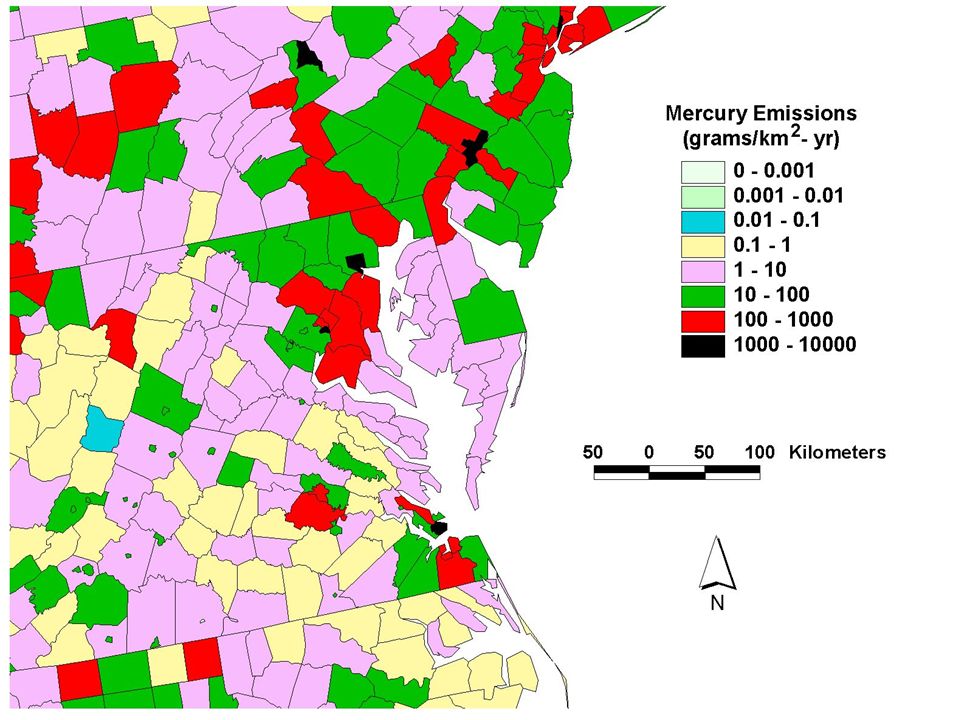
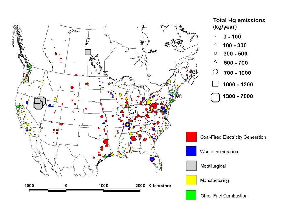
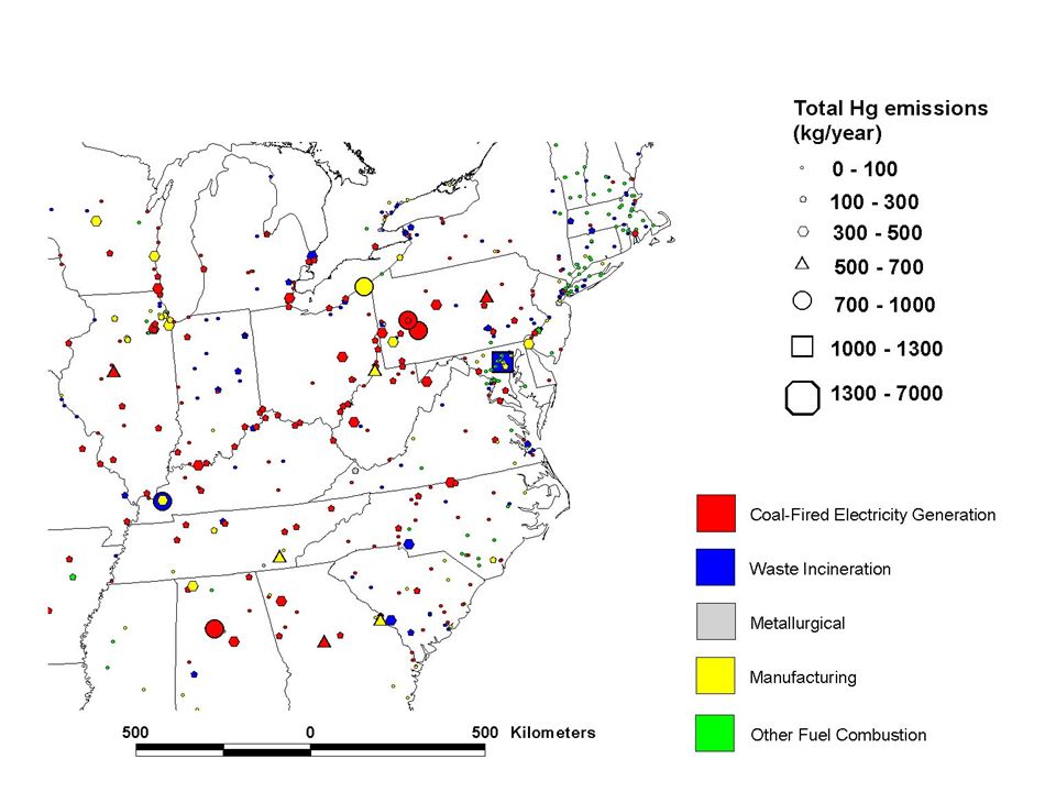
17. Geographic Distribution of Estimated Anthropogenic Mercury Emissions in the U.S. (1999) and Canada (2000)

24. Reported trends in U.S. atmospheric mercury emissions 1990-1999 (selected source categories)
Imported as pictures
(a) EPA NTI Baseline (Mobley, 2003)
(b) Hg Study Rpt to Congress (EPA, 1997)
(c) Inventory used in Cohen et al (2004)
(d) EPA 96/99 Inventory (Ryan, 2001)
(e) EPA NEI 1999 (draft) (Mobley, 2003)

25. 1995 Global Hg Emissions Inventory Josef Pacyna,NILU, Norway (2001)
And, we can’t just consider only the U.S. and Canada, sources around the world may contribute, and in fact almost assuredly do… These data come from Josef Pacyna, of NILU, in Norway.
Preliminary estimates from a few groups using global mercury models, including Ashu Dastoor of Environment Canada, suggest that global sources may account for maybe 10-25% of the mercury being deposited in the Great Lakes, but much more work needs to be done in this area…
I will be present some detailed source-receptor estimates a little later when I show you some of my modeling results.
1995 Global Hg Emissions Inventory Josef Pacyna,NILU, Norway (2001)

26. Model
Evaluation

27. Mercury Deposition Network Sites with 1996 data in the Chesapeake Bay Region

28. Modeled vs. Measured Wet Deposition at Mercury Deposition Network Site DE_02 during 1996

29. Modeled vs. Measured Wet Deposition at Mercury Deposition Network Site MD_13 during 1996

30. 1999 Results for
Chesapeake Bay

31. Geographical Distribution of 1999 Direct Deposition Contributions to the Chesapeake Bay (entire domain)

32. Geographical Distribution of 1999 Direct Deposition Contributions to the Chesapeake Bay (regional close-up)

33. Geographical Distribution of 1999 Direct Deposition Contributions to the Chesapeake Bay (local close-up)

34. Emissions and Direct Deposition Contributions from Different Distance Ranges Away From the Chesapeake Bay

35. Largest Regional Individual Sources Contributing to 1999 Mercury Deposition Directly to the Chesapeake Bay

36. Largest Local Individual Sources Contributing to 1999 Mercury Deposition Directly to the Chesapeake Bay

37. Top 25 Contributors to 1999 Hg Deposition Directly to the Chesapeake Bay

38. Deposition to the Chesapeake Bay and to its Watershed (~1999) (logarithmic graph)

39. Deposition to the Chesapeake Bay and to its Watershed (~1999) (linear graph)

40. What is Relative Importance of Hg Deposited Directly to Chesapeake Bay Surface vs. Deposition to Watershed (?)
Depends on what %
of WS-deposited Hg
makes it into the Bay...

41. Some Next Steps Use more highly resolved meteorological data grid
Expand model domain to include global sources
Simulate natural emissions and re-emissions of previously deposited Hg
Additional model evaluation exercises ... more sites, more time periods, more variables (e.g., not just wet deposition).
Sensitivity analyses and examination of atmospheric Hg chemistry in the marine boundary layer and at upper elevations...

42. Current (2004) Monitoring Sites in Chesapeake Bay Region (incomplete?)