1. (Z&B) Steps in Transport Modeling Calibration step (calibrate flow & transport model) Adjust parameter values Design conceptual model Assess uncertainty

2. Designing a Transport Model Conceptual model of the flow system Input parameters Governing equation 1D, 2D, or 3D steady-state or transient flows steady-state or transient transport Boundary conditions Initial conditions Design the grid Time step

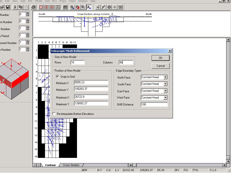
3. TMR (telescopic mesh refinement) From Zheng and Bennett TMR is used to cut out and define boundary conditions around a local area within a regional flow model.

4. GWV option for Telescopic Mesh Refinement (TMR)

7. Input Parameters for Transport Simulation Flow Transport hydraulic conductivity (K x, K y, K z ) storage coefficient (S s, S, S y ) porosity (  ) dispersivity (  L,  TH,  TV ) retardation factor or distribution coefficient 1 st order decay coefficient or half life recharge rate pumping rates source term (mass flux) All of these parameters potentially could be estimated during calibration. That is, they are potentially calibration parameters.

8. Input Parameters for Transport Simulation Flow Transport hydraulic conductivity (K x, K y, K z ) storage coefficient (S s, S, S y ) porosity (  ) dispersivity (  L,  TH,  TV ) retardation factor or distribution coefficient 1 st order decay coefficient or half life recharge rate pumping rates source term (mass flux) v = K I /  D = v  L + D d

9. We need to introduce a “law” to describe dispersion, to account for the deviation of velocities from the average linear velocity calculated by Darcy’s law. Average linear velocity True velocities

10. Figure from Freeze & Cherry (1979) Microscopic or local scale dispersion

11. Macroscopic Dispersion (caused by the presence of heterogeneities) Homogeneous aquifer Heterogeneous aquifers Figure from Freeze & Cherry (1979)

12. Dispersivity (  ) is a measure of the heterogeneity present in the aquifer. A very heterogeneous porous medium has a higher dispersivity than a slightly heterogeneous porous medium.

13. Z&B Fig. 3.24 Option 1: Assume an average uniform K value and simulate dispersion by using large values of dispersivity.

14. Field (Macro) Dispersivities Gelhar et al. 1992 WRR 28(7) Also see Appendix D In book by Spitz and Moreno (1996) A scale effect is observed.

15. Schulze-Makuch, 2005 Ground Water 43(3) Unconsolidated material

16. Tompson and Gelhar (1990) WRR 26(10) Theoretical “ideal” plume

17. Tompson and Gelhar (1990), WRR 26(10) Hydraulic conductivity field created using a random field generator Option 2: Simulate the variablity in hydraulic conductivity and use small (micro) dispersivity values.

18. See Section 14.4.2 (p. 429) in Z&B Model Application: The MADE-2 Tracer Test Injection occurs halfway between the water table and the bottom of the aquifer.

19. Injection Site Theoretical “ideal” plume MADE-2 Tracer Test

20. Generating the hydraulic conductivity field Kriging Random field generator

23. Anderson et al. (1999), Sedimentary Geology Incorporating the geology

24. Anderson et al. (1999) Sedimentary Geology Synthetic deposit of glacial outwash

25. Weissmann et al. (2002), WRR 38 (10)

26. Weissmann et al. (1999), WRR 36(6) 4 Facies

27. LLNL Site (LaBolle and Fogg, 2001) Instantaneous source Note the complex shape of the plume.

28. Option 1: Assume an average uniform K value and simulate dispersion by using large values of dispersivity. Option 2: Simulate the variablity in hydraulic conductivity and use small (micro) dispersivity values. Summary Option 2 requires detailed geological characterization that may not be feasible except for research problems.

29. Input Parameters for Transport Simulation Flow Transport hydraulic conductivity (K x, K y, K z ) storage coefficient (S s, S, S y ) porosity (  ) dispersivity (  L,  TH,  TV ) retardation factor or distribution coefficient 1 st order decay coefficient or half life recharge rate pumping rates source term (mass flux) v = K I /  D = v  L + D d

30. “…the longitudinal macrodispersivity of a reactive solute can be enhanced relative to that of a nonreactive one.” Burr et al., 1994, WRR 30(3) At the Borden Site, Burr et al. found that the value of  L needed to calibrate a transport model was 2-3 times larger when simulating a chemically reactive plume. They speculated that this additional dispersion is caused by additional spatial variability in the distribution coefficient. Research by Allen-King (NGWA Distinguished Lecturer) shows similar effects.

31. Input Parameters for Transport Simulation Flow Transport hydraulic conductivity (K x, K y, K z ) storage coefficient (S s, S, S y ) porosity (  ) dispersivity (  L,  TH,  TV ) retardation factor or distribution coefficient 1 st order decay coefficient or half life recharge rate pumping rates source term (mass flux) v = K I /  D = v  L + D d

32. Borden Plume Simulated: double-peaked source concentration (best calibration) Simulated: smooth source concentration (best calibration) Z&B, Ch. 14

33. Goode and Konikow (1990), WRR 26(10) from Z&B Transient flow field affects calibrated (apparent) dispersivity value

34. Calibrated values of dispersivity are dependent on: Heterogeneity in hydraulic conductivity (K) Heterogeneity in chemical reaction parameters (Kd and ) Temporal variability in the source term Transience in the flow field

35. Input Parameters for Transport Simulation Flow Transport hydraulic conductivity (K x, K y, K z ) storage coefficient (S s, S, S y ) porosity (  ) dispersivity (  L,  TH,  TV ) retardation factor or distribution coefficient 1 st order decay coefficient or half life recharge rate pumping rates source term (mass flux) v = K I /  D = v  L + D d

36. Common organic contaminants Source: EPA circular

37. Spitz and Moreno (1996) fraction of organic carbon

38. Spitz and Moreno ( 1996)