Download presentation
Presentation is loading. Please wait.

1
Logistic Regression Analysis Gerrit Rooks 30-03-10

2
This lecture 1.Why do we have to know and sometimes use logistic regression? 2.What is the model? What is maximum likelihood estimation? 3.Logistics of logistic regression analysis 1.Estimate coefficients 2.Assess model fit 3.Interpret coefficients 4.Check residuals 4.An SPSS example

3
Suppose we have 100 observations with information about an individuals age and wether or not this indivual had some kind of a heart disease (CHD) IDageCHD 1200 2230 3240 4251 … 98640 99651 100691
 IDageCHD …")
4
A graphic representation of the data

5
Suppose, as a researcher I am interested in the relation between age and the probability of CHD

6
To try to predict the probability of CHD, I can regress CHD on Age pr(CHD|age) = -.54 +.0218107*Age
 = *Age")
7
However, linear regression is not a suitable model for probalities. pr(CHD|age) = -.54 +.0218107*Age
 = *Age.")
8
In this graph for 8 age groups, I plotted the probability of having a heart disease (proportion)
")
9
Instead of a linear probality model, I need a non-linear one

10
Something like this

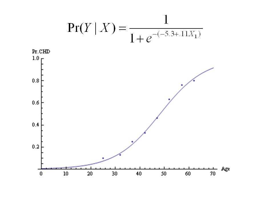
11
This is the logistic regression model

12
Predicted probabilities are always between 0 and 1 similar to classic regression analysis

13
Logistics of logistic regression 1.How do we estimate the coefficients? 2.How do we assess model fit? 3.How do we interpret coefficients? 4.How do we check regression assumptions ?

14
Logistics of logistic regression 1.How do we estimate the coefficients? 2.How do we assess model fit? 3.How do we interpret coefficients? 4.How do we check regression? assumptions ?

15
Maximum likelihood estimation Method of maximum likelihood yields values for the unknown parameters which maximize the probability of obtaining the observed set of data. Unknown parameters

16
Maximum likelihood estimation First we have to construct the likelihood function (probability of obtaining the observed set of data). Likelihood = pr(obs1)*pr(obs2)*pr(obs3)…*pr(obsn) Assuming that observations are independent
*pr(obs2)*pr(obs3)…*pr(obsn) Assuming that observations are independent.")
17
IDageCHD 1200 2230 3240 4251 … 98640 99651 100691

18
The likelihood function (for the CHD data) Given that we have 100 observations I summarize the function
 Given that we have 100 observations I summarize the function")
19
Log-likelihood For technical reasons the likelihood is transformed in the log-likelihood LL= ln[pr(obs1)]+ln[pr(obs2)]+ln[pr(obs3)]…+ln[pr(obsn)]
![Log-likelihood For technical reasons the likelihood is transformed in the log-likelihood LL= ln[pr(obs1)]+ln[pr(obs2)]+ln[pr(obs3)]…+ln[pr(obsn)]](http://images.slideplayer.com/28/9279795/slides/slide_19.jpg "Log-likelihood For technical reasons the likelihood is transformed in the log-likelihood LL= ln[pr(obs1)]+ln[pr(obs2)]+ln[pr(obs3)]…+ln[pr(obsn)]")
20
The likelihood function (for the CHD data) A clever algorithm gives us values for the parameters b0 and b1 that maximize the likelihood of this data
 A clever algorithm gives us values for the parameters b0 and b1 that maximize the likelihood of this data")
21
Estimation of coefficients: SPSS Results

23
This function fits very good, other values of b0 and b1 give worse results

24
Illustration 1: suppose we chose.05X instead of.11X

25
Illustration 2: suppose we chose.40X instead of.11X

26
Logistics of logistic regression Estimate the coefficients Assess model fit Interpret coefficients Check regression assumptions

27
Logistics of logistic regression Estimate the coefficients Assess model fit – Between model comparisons – Pseudo R 2 (similar to multiple regression) – Predictive accuracy Interpret coefficients Check regression assumptions
 – Predictive accuracy Interpret coefficients Check regression assumptions")
28
28 Model fit: Between model comparison The log-likelihood ratio test statistic can be used to test the fit of a model The test statistic has a chi-square distribution reduced model full model

29
29 Between model comparisons: likelihood ratio test reduced model full model The model including only an intercept Is often called the empty model. SPSS uses this model as a default.

30
30 Between model comparisons: Test can be used for individual coefficients reduced model full model

31
29.31 = -107,35 – 2LL(baseline)-2LL(baseline) = 136,66 This is the test statistic, and it’s associated significance Between model comparison: SPSS output
-2LL(baseline) = 136,66 This is the test statistic, and it’s associated significance Between model comparison: SPSS output")
32
32 Overall model fit pseudo R 2 Just like in multiple regression, pseudo R 2 ranges 0.0 to 1.0 – Cox and Snell cannot theoretically reach 1 – Nagelkerke adjusted so that it can reach 1 log-likelihood of model before any predictors were entered log-likelihood of the model that you want to test NOTE: R2 in logistic regression tends to be (even) smaller than in multiple regression
 smaller than in multiple regression")
33
33 Overall model fit: Classification table We correctly predict 74% of our observation

34
34 Overall model fit: Classification table 14 cases had a CHD while according to our model this shouldnt have happened.

35
35 Overall model fit: Classification table 12 cases didnt have a CHD while according to our model this should have happened.

36
Logistics of logistic regression Estimate the coefficients Assess model fit Interpret coefficients Check regression assumptions

37
Logistics of logistic regression Estimate the coefficients Assess model fit Interpret coefficients – Direction – Significance – Magnitude Check regression assumptions

38
38 Interpreting coefficients: direction We can rewrite our LRM as follows: into:

39
39 Interpreting coefficients: direction original b reflects changes in logit: b>0 -> positive relationship exponentiated b reflects the changes in odds: exp(b) > 1 -> positive relationship
 > 1 -> positive relationship")
40
40 Interpreting coefficients: direction We can rewrite our LRM as follows: into:

41
41 Interpreting coefficients: direction original b reflects changes in logit: b>0 -> positive relationship exponentiated b reflects the changes in odds: exp(b) > 1 -> positive relationship
 > 1 -> positive relationship")
42
42 Testing significance of coefficients In linear regression analysis this statistic is used to test significance In logistic regression something similar exists however, when b is large, standard error tends to become inflated, hence underestimation (Type II errors are more likely) t-distribution standard error of estimate estimate Note: This is not the Wald Statistic SPSS presents!!!
 t-distribution standard error of estimate estimate Note: This is not the Wald Statistic SPSS presents!!!")
43
Interpreting coefficients: significance SPSS presents While Andy Field thinks SPSS presents this:

44
44 3. Interpreting coefficients: magnitude The slope coefficient (b) is interpreted as the rate of change in the "log odds" as X changes … not very useful. exp(b) is the effect of the independent variable on the odds, more useful for calculating the size of an effect
 is interpreted as the rate of change in the log odds as X changes … not very useful. exp(b) is the effect of the independent variable on the odds, more useful for calculating the size of an effect.")
45
Magnitude of association: Percentage change in odds (Exponentiated coefficient i - 1.0) * 100 ProbabilityOdds 25%0.33 50%1 75%3
 * 100 ProbabilityOdds 25% %1 75%3")
46
46 For our age variable: – Percentage change in odds = (exponentiated coefficient – 1) * 100 = 12% – A one unit increase in previous will result in 12% increase in the odds that the person will have a CHD – So if a soccer player is one year older, the odds that (s)he will have CHD is 12% higher Magnitude of association
 * 100 = 12% – A one unit increase in previous will result in 12% increase in the odds that the person will have a CHD – So if a soccer player is one year older, the odds that (s)he will have CHD is 12% higher Magnitude of association")
47
Another way: Calculating predicted probabilities So, for somebody 20 years old, the predicted probability is.04 For somebody 70 years old, the predicted probability is.91

48
Checking assumptions Influential data points & Residuals – Follow Samanthas tips Hosmer & Lemeshow – Divides sample in subgroups – Checks whether there are differences between observed and predicted between subgroups – Test should not be significant, if so: indication of lack of fit

49
Hosmer & Lemeshow Test divides sample in subgroups, checks whether difference between observed and predicted is about equal in these groups Test should not be significant (indicating no difference)
")
50
Examining residuals in lR 1.Isolate points for which the model fits poorly 2.Isolate influential data points

51
Residual statistics

52
Cooks distance Means square error Number of parameter Prediction for j from all observations Prediction for j for observations excluding observation i

53
53 Illustration with SPSS Penalty kicks data, variables: – Scored: outcome variable, 0 = penalty missed, and 1 = penalty scored – Pswq: degree to which a player worries – Previous: percentage of penalties scored by a particulare player in their career

54
54 SPSS OUTPUT Logistic Regression Tells you something about the number of observations and missings

55
55 Block 0: Beginning Block this table is based on the empty model, i.e. only the constant in the model these variables will be entered in the model later on

56
56 Block 1: Method = Enter Block is useful to check significance of individual coefficients, see Field New model this is the test statistic after dividing by - 2 Note: Nagelkerke is larger than Cox

57
57 Block 1: Method = Enter (Continued) Predictive accuracy has improved (was 53%) estimates standard error estimates significance based on Wald statistic change in odds
 Predictive accuracy has improved (was 53%) estimates standard error estimates significance based on Wald statistic change in odds")
58
58 How is the classification table constructed? # cases not predicted corrrectly # cases not predicted corrrectly

59
59 How is the classification table constructed? pswqpreviousscoredPredict. prob. 18561.68 17351.41 20450.40 10420.85

60
60 How is the classification table constructed? pswqprevio us scoredPredict. prob. predict ed 18561.681 17351.410 20450.400 10420.851

Similar presentations


 Introduction to Generalized Linear Models The simplest logistic regression.>")
 Tests>")


. We now transition and begin discussion of.>")


. Goal: Fit a parsimonious model that explains variation.>")


