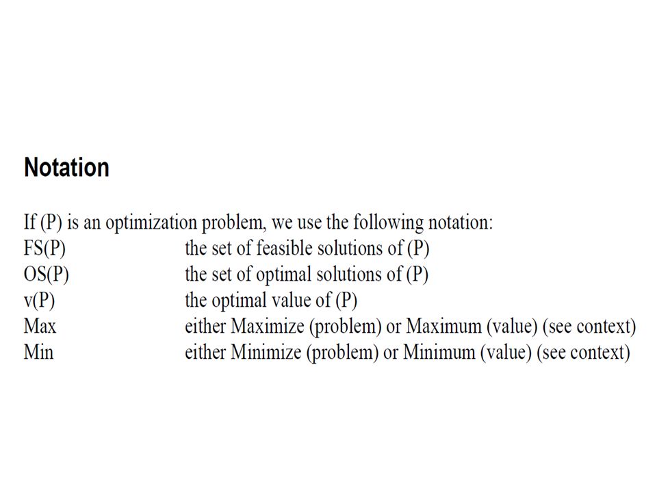
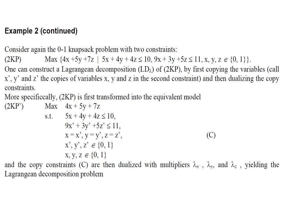
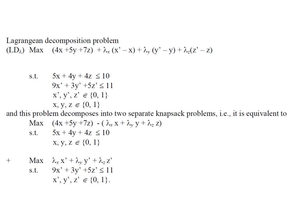
1. Lagrangean Relaxation

2. Overview Decomposition based approach. Start with Easy constraints
Complicating Constraints.
Put the complicating constraints into the objective and delete them from the constraints.
We will obtain a lower bound on the optimal solution for minimization problems.
In many situations, this bound is close to the optimal solution value.

3. An Example: Constrained Shortest Paths
Given: a network G = (N,A)
cij cost for arc (i,j)
tij traversal time for arc (i,j)
z* = Min
s. t.
Complicating constraint

4. Example
Find the shortest path from node 1 to node 6 with a transit time at most 10
$cij, tij i j
$1,10
$1,1
$1,7
$2,3
$10,3
$12,3
$2,2
$1,2
$10,1
$5,7 1 2 4 5 3 6

5. Shortest Paths with Transit Time Restrictions
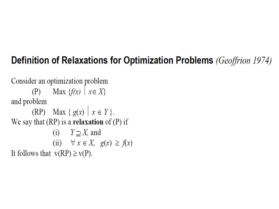
Shortest path problems are easy.
Shortest path problems with transit time restrictions are NP-hard.
We say that constrained optimization problem Y is a relaxation of problem X if Y is obtained from X by eliminating one or more constraints.
We will “relax” the complicating constraint, and then use a “heuristic” of penalizing too much transit time. We will then connect it to the theory of Lagrangian relaxations.

6. Shortest Paths with Transit Time Restrictions
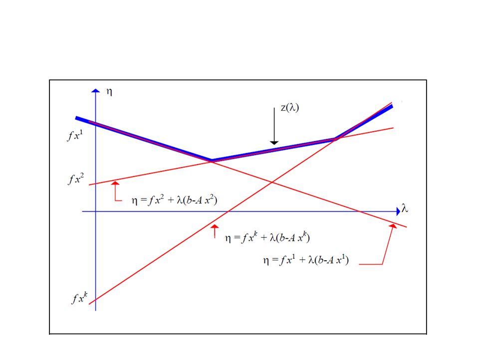
Step 1. (A Lagrangian relaxation approach). Penalize violation of the constraint in the objective function.
z(λ) = Min
Complicating constraint
Note: z*(λ) ≤ z* ∀λ ≥ 0

7. Shortest Paths with Transit Time Restrictions
Step 2. Delete the complicating constraint(s) from the problem. The resulting problem is called the Lagrangian relaxation.
Complicating constraint
L(λ) = Min
Note: L(λ) ≤ z(λ) ≤ z* ∀λ ≥ 0

8. What is the effect of varying λ?
$1,10
$1,1
$1,7
$2,3
$10,3
$12,3
$2,2
$1,2
$10,1
$5,7 1 2 4 5 3 6
Case 1: λ = 0 1 2 4 5 3 6 10 12
cij + λ tij j i
P =
P =
c(P) =
c(P) = 3
t(P) =
t(P) = 18

9. Question to class
If λ = 0, the min cost path is found. What happens to the (real) cost of the path as λ increases from 0? What path is determined as λ gets VERY large? What happens to the (real) transit time of the path as λ increases from 0?
cij + λ tij j i

10. Let λ = 1 Case 2: λ = 1 2 4 1 6 5 3 P = P = 1-2-5-6 c(P) = 5 c(P) =
$1,10
$1,1
$1,7
$2,3
$10,3
$12,3
$2,2
$1,2
$10,1
$5,7 1 2 4 5 3 6
Case 2: λ = 1 2 2 4 8 11 5 1 11 6 3 12 13 4 5 3 15
P =
P =
c(P) = 5
c(P) =
t(P) =
t(P) = 15

11. Let λ = 2 Case 3: λ = 2 2 4 1 6 5 3 P = P = 1-2-5-6 c(P) = 5 c(P) =
$1,10
$1,1
$1,7
$2,3
$10,3
$12,3
$2,2
$1,2
$10,1
$5,7 1 2 4 5 3 6
Case 3: λ = 2 3 2 4 15 21 8 1 12 6 5 19 16 6 5 3 18
P =
P =
c(P) = 5
c(P) =
t(P) =
t(P) = 15

12. And alternative shortest path when λ = 2
$1,10
$1,1
$1,7
$2,3
$10,3
$12,3
$2,2
$1,2
$10,1
$5,7 1 2 4 5 3 6 3 2 4 15 21 8 1 12 6 5 19 16 6 5 3 18
P =
P =
c(P) =
c(P) = 15
t(P) =
t(P) = 10

13. Let λ = 5 Case 4: λ = 5 2 4 1 6 5 3 P = P = 1-3-2-4-5-6 c(P) = 24
$1,10
$1,1
$1,7
$2,3
$10,3
$12,3
$2,2
$1,2
$10,1
$5,7 1 2 4 5 3 6
Case 4: λ = 5 3 2 4 15 21 8 1 12 6 5 19 16 6 5 3 18
P =
P =
c(P) = 24
c(P) =
t(P) =
t(P) = 8

14. A parametric analysis
Toll
modified cost
Cost
Transit
Time
Modified cost -10λ
0 ≤ λ ≤ ⅔
3 + 18λ 3 18
3 + 8λ
⅔ ≤ λ ≤ 2
5 + 15λ 5 15
5 + 3λ
2 ≤ λ ≤ 4.5 λ 10
4.5 ≤ λ < ∞
24 + 8λ 24 8
24 - 2λ
A lower bound on z*
The best value of λ is the one that maximizes the lower bound.

15. Costs
Modified Cost – 10λ
Transit Times λ λ

25. Problem splitting tricks

26. Embedded Network Structure
Application
Embedded Network Structure
Networks with side constraints
minimum cost flows shortest paths
Traveling Salesman Problem
assignment problem minimum cost spanning tree
Vehicle routing
assignment problem variant of min cost spanning tree
Network design
shortest paths
Two-duty operator scheduling
shortest paths minimum cost flows
Multi-time production planning
shortest paths / DPs minimum cost flows

28. Problem splitting tricks

35. Lagrangian Relaxation
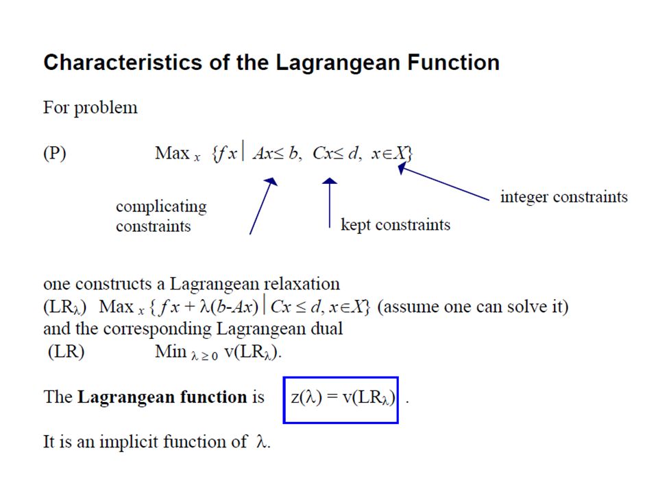
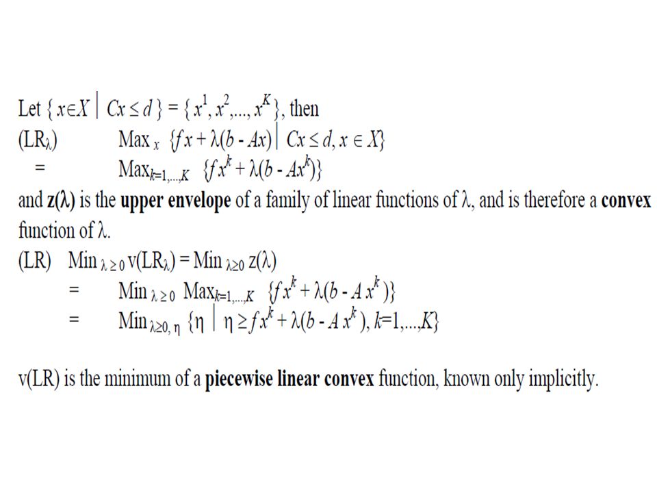
What can this be used for ?
Primary usage: Bounding ! Because it is a relaxation, the optimal value will bound the optimal value of the real problem !
Lagrangian heuristics, i.e. generate a “good” solution based on a solution to the relaxed problem.
Problem reduction, i.e. reduce the original problem based on the solution to the relaxed problem.

36. Two Problems Facing a problem we need to decide:
Which constraints to relax (strategic choice)
How to find the best lagrangean multipliers, (tactical choice)

37. Which constraints to relax
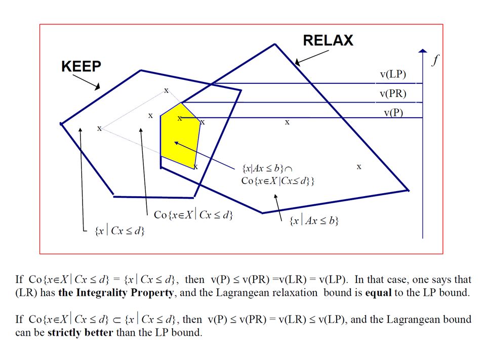
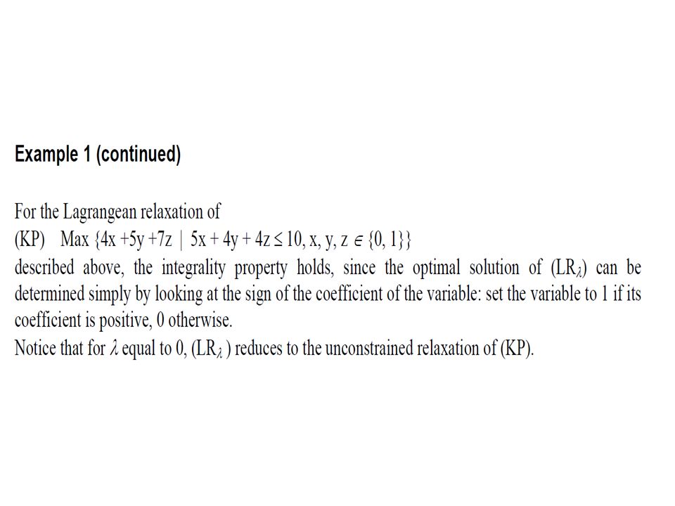
Which constraints to relax depends on two things:
Computational effort:
Number of Lagrangian multipliers
Hardness of relaxed problem to solve
Integrality of relaxed problem: If it is integral, we can only do as good as the straightforward LP relaxation !
(Integrality: the solution to relaxed problem is guaranteed to be integral.)

38. Multiplier adjustment
Two different types are given:
Subgradient optimisation
Constraint generation method
Of these, subgradient optimisation is the method of choice. This is general method which nearly always works !
Here we will only consider this Method, although more efficient (but much more complicated) adjustment methods have been suggested.

39. Linear Program
Min:
s.t.

40. Lagrangian Relaxation

41. Problem reformulation
Note: Each constraint is associated with a multiplier i.

42. The subgradient
(subgradient of multiplier i)

43. Subgradient Optimization

44. Subgradient Optimization
In the subgradient search;
Try to update UB in every iteration
Halve the step multiplier,Π, if there is no improvement in LB in the last certain number of iterations.
Stop the alpgorithm either based on the number of iterations or based on the gap between UB and LB.

45. Example: Set covering

46. Relaxed Set coverint
How can we solve this problem to optimality ???

47. Optimization Algorithm
The answer is so simple that we are reluctant calling it an optimization algorithm: Choose all x’s with negative coefficients !
What does this tell us about the strength of the relaxation ?

48. Rewritten: Relaxed Set covering
where

49. Lower bound

50. Try it out yourself
Starting with ZUB=6,=2 and i=0 for i=1,2,3, perform 3 iterations of the subgradient optimization method on the previous example problem. Please show the lower bound and multiplier values of each iteration.