1. Population Models Modeling and Simulation I-2012

2. Content 1. Basic Population Model 2. One population A.Exponential growth B.Logistic growth C.Linear growth D.Stochastic Population Dynamics Modeling E.Real Human Populations 3. Two populations A.Lotka-Volterra B.Kolgomrov

3. What is Demography? The scientific study of the changing size, composition and spatial distribution of a human population and the processes which shape them. Is concerned with: Population size Population growth or decline Population processes Population distribution Population structure Population characteristics 1. Basic Population Model

4. Basic Population Model N(t) N(t): Population size Number of individuals in the population

5. Historical Context The starting point for population growth models is The Principle of Population, published in 1798 by Thomas R. Malthus (1766-1834). In it he presented his theories of human population growth and relationships between over-population and misery. The model he used is now called the exponential model of population growth. In 1846, Pierre Francois Verhulst, a Belgian scientist, proposed that population growth depends not only on the population size but also on the effect of a “carrying capacity” that would limit growth. His formula is now called the "logistic model" or the Verhulst model.

6. Recent Developments Most recently, the logistic equation has been used as part of exploration of what is called "chaos theory". Most of this work was collected for the first time by Robert May in a classic article published in Nature in June of 1976. Robert May started his career as a physicist but then did his post-doctoral work in applied mathematics. He became very interested in the mathematical explanations of what enables competing species to coexist and then in the mathematics behind populations growth. Stochastic Population Dynamics Modeling

7. 2. Relevant Models Exponential growth Logistic growth Linear growth Stochastic Population Dynamics Modeling

8. A. Exponential growth pop. size at time t+  t = pop. size at time t + growth increment N(t+  t) = N(t ) +  N Hypothesis:  N = r N  t r - rate constant of growth

9. Differential equation for exponential growth

10. 02468101214161820 0 1 2 3 4 5 6 7 8 9 10 Time - t N(t) Exponential growth r=0.1

11. Exponential growth in discrete time N t+1 = N t + r N t N t+1 = (1+r) N t N t = (1+r) t N 0

12. Exponential decline r - mortality rate

13. Time – t N(t) Exponential decline r=0.1

14. B. Logistic growth model Relies on the hypothesis that population growth is limited by environmental capacity K – environmental capacity Differential equation for Logistic growth

15. As this shows, the curve produced by the logistic difference equation is S-shaped. Initially there is an exponential growth phase, but as growth gets closer to the carrying capacity (more or less at time step 37 in this case), the growth slows down and the population asymptotically approaches capacity. N t+1 = N t + ((K – N t )/K)*r*N t N t+1 = ((K – N t )/K)*(1 + r)*N t Logistic growth in discrete time

16. For some parameter this model can exhibit periodic or chaotic behavior

17. Stochastic vs. deterministic So far, all models we’ve explored have been “deterministic” Their behavior is perfectly “determined” by the model equations Alternatively, we might want to include “stochasticity”, or some randomness to our models Stochasticity might reflect: Environmental stochasticity Demographic stochasticity C. Stochastic Population Modelling

18. Demographic stochasicity We often depict the number of surviving individuals from one time point to another as the product of Numbers at time t (N(t)) times an average survivorship This works well when N is very large (in the 1000’s or more) For instance, if I flip a coin 1000 times, I’m pretty sure that I’m going to get around 500 heads (or around p * N = 0.5 * 1000) If N is small (say 10), I might get 3 heads, or even 0 heads The approximation N = p * 10 doesn’t work so well

19. Why consider stochasticity? Stochasticity generally lowers population growth rates “Autocorrelated” stochasticity REALLY lowers population growth rates Allows for risk assessment What’s the probability of extinction What’s the probability of reaching a minimum threshold size

20. Mechanics: Adding Environmental Stochasticity In stochastic models, we presume that the dynamic equation reflect the evolution of a a probability distribution, so that : Where v(t) is some random variable with a mean 0.

21. Density-Independent Model Deterministic Model: We can predict population size 2 time steps into the future: Or any ‘n’ time steps into the future:

22. Adding Stochasicity Presume that varies over time according to some distribution N(t+1)= (t)N(t) Each model run is unique We’re interested in the distribution of N(t)s

23. Why does stochasticity lower overall growth rate Consider a population changing over 500 years: N(t+1)= (t)N(t) During “good” years, = 1.16 During “bad” years, = 0.86 The probability of a good or bad year is 50% N(t+1)=[ t t-1 t-2 ….  2 1 o ]N(0) The “arithmetic” mean of ( A )equals 1.01 (implying slight population growth)

24. Model Result There are exactly 250 “good” and 250 “bad” years This produces a net reduction in population size from time = 0 to t =500 The arithmetic mean doesn’t tell us much about the actual population trajectory!

25. Why does stochasticity lower overall growth rate N(t+1)=[ t t-1 t-2 ….  2 1 o ]N(0) There are 250 good and 250 bad N(500)=[1.16 250 x 0.86 250 ]N(0 ) N(500)=0.9988 N(0) Instead of the arithmetic mean, the population size at year 500 is determined by the geometric mean: The geometric mean is ALWAYS less than the arithmetic mean

26. Calculating Geometric Mean Remember: ln ( 1 x 2 x 3 x 4 )=ln( 1 )+ln( 2 )+ln( 3 )+ln( 4 ) So that geometric mean G = exp(ln( t )) It is sometimes convenient to replace ln( ) with r

27. Mean and Variance of N(t) If we presume that r is normally distributed with mean r and variance  2 Then the mean and variance of the possible population sizes at time t equals

28. Probability Distributions of Future Population Sizes r ~ N(0.08,0.15)

29. Population Trends World Population Growth Billions of people 1820 1 billion 1930 2 billion 2000 6.1 billion 3. Real Human Populations

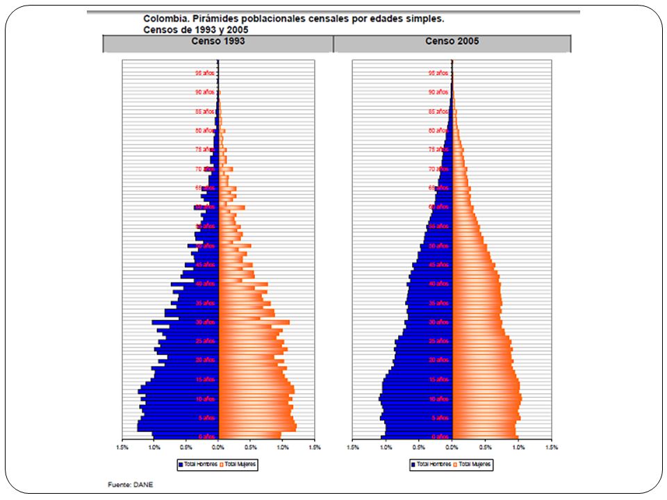
30. 1/9/2007 Population perspective 30 Population pyramids

31. 1/9/2007 Population perspective 31

32. China’s Age Distribution by age and sex, 1964, 1982, and 2000 From Figure 6. China’s Population by Age and Sex, 1964, 1982, and 2000 from Nancy E. Riley, China’s Population: New trends and challenges. Population Bulletin 2004: 59(2);21. Original sources: Census Bureau, International Data Base (www.census.gov/ipc/www/idbnew.html, accessed April 7, 2004); and tabulations from the China 2000 Census.

33. 33

34. Millions 77M born 1980 - 1999 77M born 1980 - 1999 76M born 1945 - 1964 “Baby Boomers” 76M born 1945 - 1964 “Baby Boomers” U.S. Population Distribution by Age Segments for 2004

35. Births and Selected Age Groups in the United States

36. 36

37. 37

38. 38

39. 39

40. 40

41. Total nacional 41.468.384 1. Censo 2005 DANE

42. 2005 205020002025 http:// www.imsersomayores.csic.es/internacional/iberoamerica/colombia/indicadores.html http://www.dane.gov.co 2005

44. Censos DANE 45.532.558 (Julio) CIA 44.205.293 (enero) http://www.imsersomayores.csic.es Proyecciones

45. http:// www.imsersomayores.csic.es/internacional/iberoamerica/colombia/indicadores.html AñoPoblación totalPoblación mayor de 60 200042.321.0002.900.000 202559.758.0008.050.000 205070.351.00015.440.000

46. Densidad de Población Colombia http://es.wikipedia.org/wiki/Demografía_de_Colombia

47. Población 44,205,293 (July 2010 est.) country comparison to the world: 2828 2. Datos del CIA World Factbook 2010

48. Esperanza de vida total population: 74.31 years country comparison to the world: 9696 male: 70.98 years female: 77.84 years (2010 est.)