1. Modeling Distributions
Chapter 3
Modeling Distributions
of Data

2. Section 3.2
Normal Distributions

3. Normal Curve
The Normal curve has a distinctive, symmetric, single-
peaked bell shape.
Normal curves have special properties
Normal curves describe Normal distributions

4. They are important because
Normal distributions.... play an important role and are rather special, but not at all "normal", "average" or "natural"!
They are important because
They are good descriptions for distributions of real data
They are good approximations to results of chance outcomes
Many statistical inference procedures are based on them

5. We can locate the standard deviation of the distribution by eye on the curve!
Figure 3.12
Two Normal curves. The standard deviation fixes the spread of a Normal curve.

6. Normal curves...
Knowing the mean and standard deviation completely specifies the curve.
The mean fixes the center
The standard deviation determines its shape
Changing the mean does not change its shape, only its location on the x-axis
Changing the standard deviation does change the shape, a smaller deviation is less spread out and more sharply peaked

7. Normal curves...
Are symmetric, bell-shaped curves that have these properties
completely described by giving its mean and its standard deviation
the mean determines the center of the distribution, it is located at the center of symmetry of the curve
the standard deviation determines the shape of the curve, it is the distance from the mean to the change-of-curvature points on either side

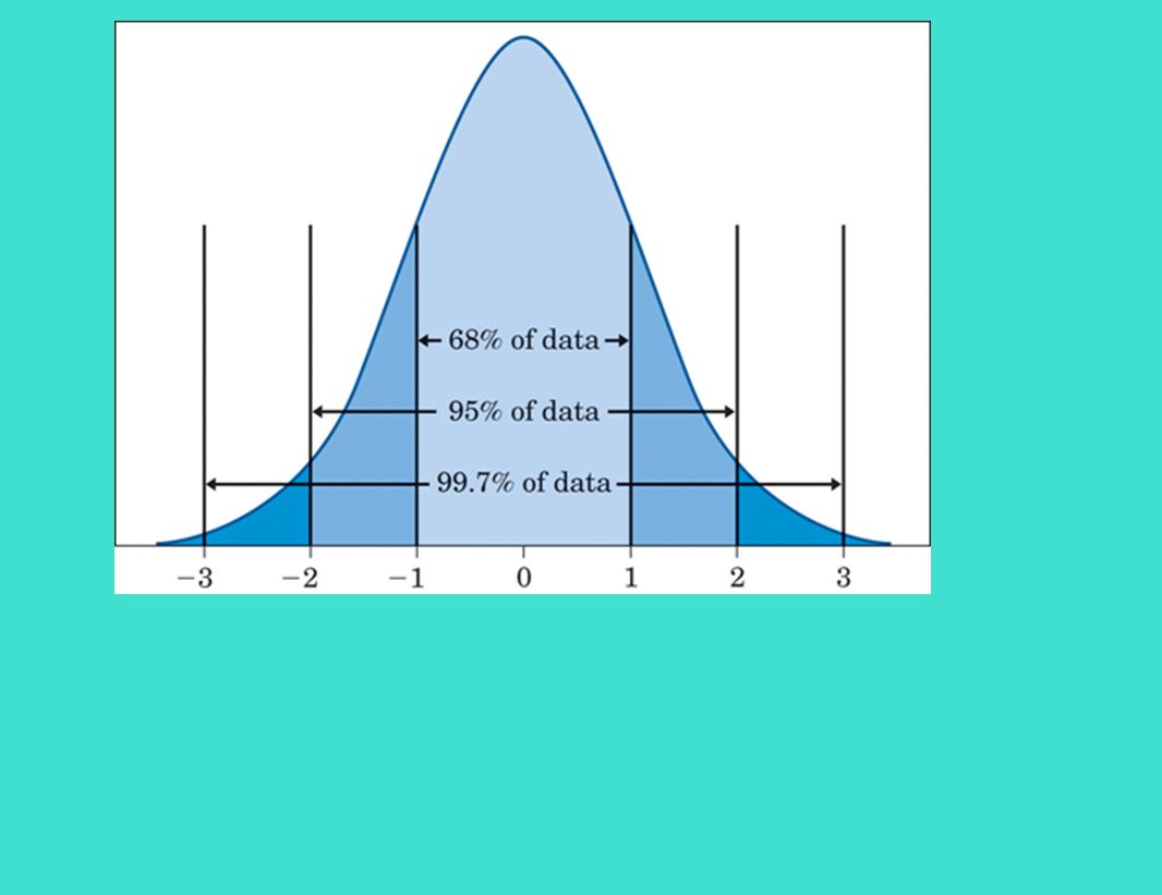
8. The Empirical Rule (aka 68-95-99.7 Rule)
In any Normal distribution, approximately
68% of the observations fall within one standard deviation of the mean
95% of the observations fall within two standard deviations of the mean
99.7% of the observations fall within three standard deviations of the mean

10. Figure 3.14
The 68–95–99.7 rule shows that 84% of any Normal distribution lies to the left of the point one standard deviation above the mean. Here, this fact is applied to SAT scores.

11. Before we stated that
z =
__x - mean __
standard deviation
Now
μ (mu) = mean of a density curve
σ (small sigma) = standard deviation of a density curve
We use these to represent a population distribution
So z =
x-μ σ

12. The standard Normal distribution
the Normal distribution with mean 0 and standard deviation 1
z has the standard Normal distribution...

13. The Empirical Rule states that 68% of observations fall between z = -1 and z = 1.
How can we find the percentage of observations between z = and z = 1.25?

14. The standard Normal table (the z-score table) gives us areas under the Normal curve.

15. Find the proportions of observations from the standard Normal distribution that are (a) less than and (b) greater than 0.81.
(a)
z-scores.xps

16. (b)
z-scores.xps

17. Now find the area between -1.25 and 0.81
The area under the standard Normal curve 
between z = and z = 0.81 is
1 - ( ) = =

18. Finding z-scores from percentiles
z-scores.xps

19. To do problems with a Normal distribution instead of the 
Standard Normal distribution, first standardize values by 
finding z-scores.
Practice 3.2.xps

21. Attachments
z-scores.xps
Practice 3.2.xps