1. Office: E409 Tel: 3620623(office), 3620620(T.A.) Statistics for Business Instructor: Dr. Peng Xiaoling T.A. : Miss Li Jianxia Email: xlpeng@uic.edu.hk (Instructor)xlpeng@uic.edu.hk lemonli@uic.edu.hk (T.A.)lemonli@uic.edu.hk Website: www.uic.edu.hk/~xlpengwww.uic.edu.hk/~xlpeng

2. What is Statistics? Statistics is the science of collecting, organizing, presenting, analyzing, and interpreting numerical data to assist in making more effective decisions.

4. Statistics is very useful to your future career  Government officials use conclusions drawn from the latest data on unemployment and inflation to make policy decisions.  Financial planners use recent trends in stock market prices to make investment decisions.

5. General Information (Textbook) Bowerman and O’Connell, Business Statistics in Practice, McGraw-Hill. (Software) SPSS 17.0 (Assessment grade system) A and A- (Not more than 10%), A, A-, B+, B, B- (Not more than 65%).

6. Assessment ~ Continuous Assessment (50%) ~ Homework (30%) Six or more sets of home works and several quizzes on class ~ Mid-term test (20%) ~ Final examination (50%)

7. Outline of the course Introduction to Statistics Descriptive Statistics Probability and Random Variables Sampling Distributions Confidence Interval and Hypothesis Testing Statistical Inferences Based on Two Samples Some Optional Topics (Linear Regression)

8. Chapter 1 An introduction to Business Statistics  Populations and Samples  Sampling a Population of Existing Units  Sampling a Process  An Introduction to Survey Sampling

9. Populations and Samples PopulationA set of existing units (people, objects, or events) SampleA selected subset of the units of a population Examples of Population: All UIC graduates. All Lincoln Town Cars that were produced last year. All Lincoln Town Cars that were produced last year. Population Size, N Sample Size, n

10. Population vs. Sample a b c d e f g h i j k l m n o p q r s t u v w x y z PopulationSample b c g i n o r u y Measures used to describe a population are called variables. Measures computed from sample data are called statistics.

11. An examination of the entire population of measurements. Census( 普查 ) Note: Census usually too expensive, too time consuming, and too much effort for a large population. A selected subset of the units of a population. Sample Population Sample For example, a university graduated 8,742 students a. This is too large for a census. b. So, we select a sample of these graduates and learn their annual starting salaries.

12. Questions: What ’ s the population & sample? A pollster asks 30 adults at the mall about their shopping preferences. Fox News does a poll, and reports the opinions of the 2500 people who called in. Researchers test out a new cancer drug on 100 men with lung cancer.

13. Chapter 1 Introduction A measurable characteristic of the population. Variable We carry out a measurement to assign a value of a variable to each population unit. Type of variables: Quantitative (numerical) Qualitative (Categorical)

14.  The variable is said to be quantitative or :  The variable is said to be quantitative or numerical: Measurements that represent quantities (for example, “how much” or “how many”). For example, annual starting salary is quantitative, age and number of children is also quantitative Number of children in a family Balance in your bank account Minutes remaining in class

15.  The variable is said to be qualitative or categorical: A descriptive category to which a population unit belongs. For example, a person’s gender and whether a person who purchases a product is satisfied with the product are qualitative.

16. Chapter 1 Introduction Nominative: Nominative: Identifier or name Identifier or name Unranked categorization Unranked categorization Example: gender, car color Example: gender, car color Ordinal (can be compared): Ordinal (can be compared): All characteristics of nominative plus… All characteristics of nominative plus… Rank-order categories Rank-order categories Ranks are relative to each other Ranks are relative to each other Example: Low (1), moderate (2), or high (3) risk Example: Low (1), moderate (2), or high (3) risk There are two types of qualitative variables:

17. Descriptive Statistics Vs. Inferential Statistics Types of Statistics

18. Chapter 1 Introduction For example, for a set of annual starting salaries, we want to know: For example, for a set of annual starting salaries, we want to know: How much to expect How much to expect What is a high versus low salary What is a high versus low salary How much the salaries differ from each other How much the salaries differ from each other If the population is small enough, could take a census and not have to sample and make any statistical inferences If the population is small enough, could take a census and not have to sample and make any statistical inferences But if the population is too large, then ………. But if the population is too large, then ………. The science of describing the important aspects of a set of measurements Descriptive statistics

19. Descriptive Statistics Collect data e.g. Survey Present data e.g. Tables and graphs Characterize data e.g. Sample mean =

20. Chapter 1 Introduction Statistical Inference The science of using a sample of measurements to make generalizations about the important aspects of a population of measurements. For example, use a sample of starting salaries to estimate the important aspects of the population of starting salaries For example, use a sample of starting salaries to estimate the important aspects of the population of starting salaries There is a criteria on how to choose a sample: the information contained in a sample is to accurately reflect the population under study.

21. Inferential Statistics Estimation e.g.: Estimate the population mean weight using the sample mean weight Hypothesis testing e.g.: Test the claim that the population mean weight is 120 pounds Drawing conclusions and/or making decisions concerning a population based on sample results.

22. Inferential Statistics Analysis of relationship e.g.: Does the rate of growth of the money supply influence the inflation rate? Forecasting e.g.: Prediction of future interest rates

23. 1.2 Sampling a Population of Existing Units For example, randomly pick two different people from a group of 15: For example, randomly pick two different people from a group of 15: Number the people from 1 to 15; and write their numbers on 15 different slips of paper Number the people from 1 to 15; and write their numbers on 15 different slips of paper Thoroughly mix the papers and randomly pick two of them Thoroughly mix the papers and randomly pick two of them The numbers on the slips identifies the people for the sample The numbers on the slips identifies the people for the sample Each population unit has the same chance of being selected as every other unit Each population unit has the same chance of being selected as every other unit Each possible sample (of the same size) has the same chance of being selected Each possible sample (of the same size) has the same chance of being selected A random sample is a sample selected from a population so that: Random sample

24. Chapter 1 Introduction Guarantees a sample of different units Guarantees a sample of different units Each sampled unit contributes different information Each sampled unit contributes different information Sampling without replacement is the usual and customary sampling method Sampling without replacement is the usual and customary sampling method A sampled unit is withheld from possibly being selected again in the same sample Sample without replacement The unit is placed back into the population for possible reselection However, the same unit in the sample does not contribute new information Replace each sampled unit before picking next unit Sample with replacement

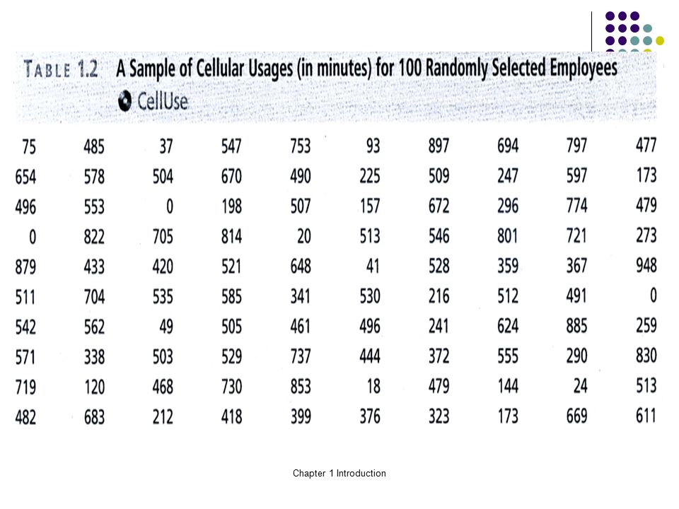
25. Chapter 1 Introduction Example 1.1 Example 1.1 The Cell Phone Case: Estimating Cell Phone Costs The bank has 2,136 employees on a 500-minute-per- month plan with a monthly cost of $50. The bank will estimate its cellular cost per minute for this plan by examining the number of minutes used last month by each of 100 randomly selected employees on this 500-minute plan. According to the cellular management service, if the cellular cost per minute for the random sample of 100 employees is over 18 cents per minute, the bank should benefit from automated cellular management of its calling plans.

26. Chapter 1 Introduction  In order to randomly select the sample of 100 cell phone users, the bank will make a numbered list of the 2,136 users on the 500-munite plan. This list is called a frame.  The bank can use a random number table, such as Table 1.1(a), or a computer software package, such as Table 1.1 (b), to select the needed sample.  The 100 cellular-usage figures are given in Table 1.2.

27. Chapter 1 Introduction

29. Approximately Random Samples Sometimes it is not possible to list and thus number all the units in a population. In such a situation we often select a systematic sample, which approximates a random sample. A Systematic Sample Randomly enter the population and systematically sample every kth unit.

30. Chapter 1 Introduction Example 1.2 Example 1.2 The Marketing Research Case: Rating a New Bottle Design To study consumer reaction to a new design, the brand group will use “mall intercept method” in which shoppers at a large metropolitan shopping mall are intercepted and asked to participate in a consumer survey. The questionnaire are shown in Figure 1.1. Each shopper will be exposed to the new bottle design and asked to rate the bottle image using a 7-point “Likert scale.” To study consumer reaction to a new design, the brand group will use “mall intercept method” in which shoppers at a large metropolitan shopping mall are intercepted and asked to participate in a consumer survey. The questionnaire are shown in Figure 1.1. Each shopper will be exposed to the new bottle design and asked to rate the bottle image using a 7-point “Likert scale.” We select a systematic sample. To do this, every 100 th shopper passing a specified location in the mall will be invited to participate in the survey. During a Tuesday afternoon and evening, a sample of 60 shoppers is selected by using the systematic sampling process. The 60 composite scores are given in Table 1.3. From this table, we can estimate that 95 percent of the shoppers would give the bottle design a composite score of at least 25. We select a systematic sample. To do this, every 100 th shopper passing a specified location in the mall will be invited to participate in the survey. During a Tuesday afternoon and evening, a sample of 60 shoppers is selected by using the systematic sampling process. The 60 composite scores are given in Table 1.3. From this table, we can estimate that 95 percent of the shoppers would give the bottle design a composite score of at least 25.

31. Chapter 1 Introduction

32. Voluntary response sample Participants select themselves to be in the sample Participants “self-select” For example, calling in to vote on American Idol For example, calling in to vote on American Idol Commonly referred to as a “non-scientific” sample Commonly referred to as a “non-scientific” sample Usually not representative of the population Over-represent individuals with strong opinions Over-represent individuals with strong opinions Usually, but not always, negative opinions Usually, but not always, negative opinions Another Sampling Method

33. Chapter 1 Introduction 1.3 Sampling a Process Process A sequence of operations that takes inputs (labor, raw materials, methods, machines, and so on) and turns them into outputs (products, services, and the like) Inputs Process Outputs

34. Chapter 1 Introduction Cars will continue to be made over time For example, all automobiles of a particular make and model, for instance, the Lincoln Town Car  The “population” from a process is all output produced in the past, present, and the yet-to-occur future. Processes produce output over time

35. Chapter 1 Introduction Example 1.3 Example 1.3 The Coffee Temperature Case: Monitoring Coffee Temperatures Monitoring Coffee Temperatures This case concerns coffee temperatures at a fast-food restaurant. To do this, the restaurant personnel measure the temperature of the coffee being dispensed (in degrees F) at half-hour intervals from 10 A.M. to 9:30 P.M. on a given day. Data is list on Table 1.7.  A process is in statistical control if it does not exhibit any unusual process variations.  To determine if a process is in control or not, sample the process often enough to detect unusual variations  A runs plot is a graph of individual process measurements over time. Figure 1.3 shows a runs plot of the temperature data.

36. Chapter 1 Introduction

37. Figure 1.3 Runs Plot of Coffee Temperatures: The Process is in Statistical Control.

38. Chapter 1 Introduction Over time, temperatures appear to have a fairly constant amount of variation around a fairly constant level The temperature is expected to be at the constant level shown by the horizontal blue line Sometimes the temperature is higher and sometimes lower than the constant level About the same amount of spread of the values (data points) around the constant level The points are as far above the line as below it The data points appear to form a horizontal band So, the process is in statistical control Coffee-making process is operating “consistently” Results

39. Chapter 1 Introduction Because the coffee temperature has been and is presently in control, it will likely stay in control in the future Because the coffee temperature has been and is presently in control, it will likely stay in control in the future If the coffee making process stays in control, then coffee temperature is predicted to be between 152 o and 170 o F If the coffee making process stays in control, then coffee temperature is predicted to be between 152 o and 170 o F In general, if the process appears from the runs plot to be in control, then it will probably remain in control in the future In general, if the process appears from the runs plot to be in control, then it will probably remain in control in the future The sample of measurements was approximately random The sample of measurements was approximately random Future process performance is predictable Future process performance is predictable Remark

40. Chapter 1 Introduction 1.4 An Introduction to Survey Sampling Already know some sampling methods Also called sampling designs, they are: Random sampling The focus of this book Systematic sampling Voluntary response sampling But there are other sample designs: Stratified random sampling Cluster sampling

41. Systematic Sampling

42. Chapter 1 Introduction More on Systematic Sampling  Want a sample containing n units from a population containing N units  Take the ratio N/n and round down to the nearest whole number Call the rounded result k  Randomly select one of the first k elements from the population list  Step through the population from the first chosen unit and select every k th unit  This method has the properties of a simple random sample, especially if the list of the population elements is a random ordering

43. Chapter 1 Introduction Stratified Random Sample Divide the population into non-overlapping groups, called strata, of similar units Separately, select a random sample from each and every stratum Combine the random samples from each stratum to make the full sample Population Divided into 4 strata Sample

44. Appropriate when the population consists of two or more different groups so that: The groups differ from each other with respect to the variable of interest Units within a group are similar to each other For example, divide population into strata by age, gender, income, etc Stratified Random Sample

45. Chapter 1 Introduction Cluster Sampling “Cluster” or group a population into subpopulations Cluster by geography, time, and so on… Each cluster is a representative small-scale version of the population (i.e. heterogeneous group) A simple random sample is chosen from each cluster Combine the random samples from each cluster to make the full sample Population divided into 16 clusters. Randomly selected clusters for sample

46. There are different sections or regions in the area with respect to the variable of interest A random sample of the cluster Cluster Sampling Appropriate for populations spread over a large geographic area so that…

47. Chapter 1 Introduction Sampling Problems  Random sampling should eliminate bias  But even a random sample may not be representative because of: Under-coverage Too few sampled units or some of the population was excluded Non-response When a sampled unit cannot be contacted or refuses to participate Response bias Responses of selected units are not truthful

48. Chapter 2 Descriptive Statistics  Describing the Shape of a Distribution  Describing Central Tendency  Measures of Variation  Percentiles, Quartiles, and Box-and- Whiskers Displays  Describing Qualitative Data  Using Scatter Plots*  Weighted Means and Grouped Data

49. Chapter 2 Descriptive Statistics 2.1 Describing the Shape of a Distribution  To know what the population looks like, find the “shape” of its distribution  Picture the distribution graphically by any of the following methods: Stem-and-leaf display Stem-and-leaf display Frequency distributions Frequency distributions Histogram Histogram Dot plot Dot plot

50. Chapter 2 Descriptive Statistics Stem-and-leaf Display The purpose of a stem-and-leaf display is to see the overall pattern of the data, by grouping the data into classes The purpose of a stem-and-leaf display is to see the overall pattern of the data, by grouping the data into classes To see: To see: the variation from class to class the variation from class to class the amount of data in each class the amount of data in each class the distribution of the data within each class the distribution of the data within each class Best for small to moderately sized data distributions Best for small to moderately sized data distributions

51. Chapter 2 Descriptive Statistics Example 2.1 Example 2.1 The Car Mileage Case  In this case study, we consider a tax credit offered by the federal government to automakers for improving the fuel economy of midsize cars.  To find the combined city and highway mileage estimate for a particular car model, the EPA tests a sample of cars.  Table 2.1 presents the sample of 49 gas mileages that have been obtained by the new midsize model.

52. Chapter 2 Descriptive Statistics 30.830.932.032.332.6 31.730.431.432.731.4 30.132.530.831.231.8 31.630.332.830.631.9 32.131.332.031.732.8 33.332.131.531.431.5 31.332.532.432.231.6 31.031.831.031.530.6 32.030.429.831.732.2 32.430.531.130.6 Table 2.1 A sample of 49 mileages

53. Chapter 2 Descriptive Statistics The stem-and-leaf display of car mileages: 29 8 30 13445666889 31 00123344455566777889 32 0001122344556788 33 3 29 + 0.8 = 29.8 33 + 0.3 = 33.3

54. Chapter 2 Descriptive Statistics Another display of the same data using more classes  Starred classes (*) extend from 0.0 to 0.4  Unstarred classes extend from 0.5 to 0.9 29 8 30* 1344 30 5666889 31* 001233444 31 55566777889 32* 0001122344 32 556788 33* 3

55. Chapter 2 Descriptive Statistics  Looking at the last stem-and-leaf display, the distribution appears almost “symmetrical” The upper portion of the display… The upper portion of the display… Stems 29, 30*, 30, and 31* Stems 29, 30*, 30, and 31* … is almost a mirror image of the lower portion of the display … is almost a mirror image of the lower portion of the display Stems 31, 32*, 32, and 33* Stems 31, 32*, 32, and 33* But not exactly a mirror reflection But not exactly a mirror reflection Maybe slightly more data in the lower portion than in the upper portion Maybe slightly more data in the lower portion than in the upper portion  Later, we will call this a slightly “left- skewed” distribution

56. Chapter 2 Descriptive Statistics Constructing a Stem-and-Leaf Display 1.Decide what units will be used for the stems and the leaves. As a general rule, choose units for the stems so that there will be somewhere between 5 and 20 stems. 2.Place the stems in a column with the smallest stem at the top of the column and the largest stem at the bottom. 3.Enter the leaf for each measurement into the row corresponding to the proper stem. The leaves should be single-digit numbers (rounded values). 4.If desired, rearrange the leaves so that they are in increasing order from left to right.

57. Chapter 2 Descriptive Statistics Example 2.2 Example 2.2 The Payment Time Case: Reducing Payment Times In order to assess the effectiveness of the system, the consulting firm will study the payment times for invoices processed during the first three months of the system’s operation. During this period, 7,823 invoices are processed using the new system. To study the payment times of these invoices, the consulting firm numbers the invoices from 0001 to 7823 and uses random numbers to select a random sample of 65 invoices. The resulting 65 payment times are given in Table 2.2

58. Chapter 2 Descriptive Statistics 2229161518171213171615 1917102115141718122014 1615162022142519231519 1823221616191318242426 1318171524151714181721 16212519202716171621 Table 2.2 A Sample of Payment Times (in Days) for 65 Randomly Selected Invoices.

59. Chapter 2 Descriptive Statistics 1 10 0 2 11 0 4 12 00 7 13 000 11 14 0000 18 15 0000000 27 16 000000000 (8) 17 00000000 30 18 000000 24 19 00000 19 20 000 16 21 000 13 22 000 10 23 00 8 24 000 5 25 00 3 26 0 2 27 0 1 28 1 29 0 Shorter tail Longer tail The leftmost column of numbers are the numbers are the amounts of values in each stem The number 8 in parentheses indicates that there are 8 payments in the stem for 17 daysThe number 8 in parentheses indicates that there are 8 payments in the stem for 17 days The number 27 (no parentheses) indicates that there are 27 payments made in 16 or less daysThe number 27 (no parentheses) indicates that there are 27 payments made in 16 or less days

60. Chapter 2 Descriptive Statistics  Looking at this display, we see that all of the sampled payment times are substantially less than the 39-day typical payment time of the former billing system.  The stem-and-leaf display do not appear symmetrical. The “tail” of the distribution consisting of the higher payment times is longer than the “tail” of the distribution consisting of the smaller payment times.  We say that the distribution is skewed with a tail to the right.

61. Chapter 2 Descriptive Statistics Frequency Distribution and Histogram A frequency distribution is a list of data classes with the count or “frequency” of values that belong to each class “Classify and count” “Classify and count” The frequency distribution is a table The frequency distribution is a table Show the frequency distribution in a histogram The histogram is a picture of the frequency distribution The histogram is a picture of the frequency distribution See Examples 2.2, The Payment Time Case

62. Chapter 2 Descriptive Statistics Constructing a Frequency Distribution  Steps in making a frequency distribution: 1.Determine the number of classes K 2.Determine the class length 3.Set the starting value for the classes, that is, the distribution “floor” 4.Calculate the class limits 5.Setup all the classes  Then tally the data into the K classes and record the frequencies

63. Chapter 2 Descriptive Statistics Number of Classes K  Group all of the n data into K number of classes  K is the smallest whole number for which 2 K  n  In Examples 2.2, n = 65 For K = 6, 2 6 = 64, < n For K = 7, 2 7 = 128, > n So use K = 7 classes

64. Chapter 2 Descriptive Statistics Class Length  Class length L is the step size from one to the next  In Examples 2.2, The Payment Time Case, the largest value is 29 days and the smallest value is 10 days, so  Arbitrarily round the class length up to 3 days/class

65. Chapter 2 Descriptive Statistics Starting the Classes  The classes start on the smallest data value This is the lower limit of the first class  The upper limit of the first class is smallest value + (L – 1) In the example, the first class starts at 10 days and goes up to 12 days  The second class starts at the upper limit of the first class + 1 and goes up (L – 1) more The second class starts at 13 days and goes up to 15 days  And so on

66. Chapter 2 Descriptive Statistics Tallies and Frequencies: Example 2.2 Classes (days)TallyFrequency 10 to 12|||3 13 to 15 |||| 14 16 to 18 ||| 23 19 to 21 || 12 22 to 24 ||| 8 25 to 27 |||| 4 28 to 30| 1 65 |||| Check: All frequencies must sum to n

67. Chapter 2 Descriptive Statistics  The relative frequency of a class is the proportion or fraction of data that is contained in that class Calculated by dividing the class frequency by the total number of data values Relative frequency may be expressed as either a decimal or percent A relative frequency distribution is a list of all the data classes and their associated relative frequencies Relative Frequency

68. Chapter 2 Descriptive Statistics Relative Frequency: Example 2.2 Classes (days)FrequencyRelative Frequency 10 to 123 3/65 = 0.0462 13 to 1514 14/65 = 0.2154 16 to 18230.3538 19 to 21120.1846 22 to 2480.1231 25 to 2740.0615 28 to 30 10.0154 651.0000 Check: All relative frequencies must sum to 1

69. Chapter 2 Descriptive Statistics Histogram  A graph in which rectangles represent the classes  The base of the rectangle represents the class length  The height of the rectangle represents the frequency in a frequency histogram, or the frequency in a frequency histogram, or the relative frequency in a relative frequency histogram the relative frequency in a relative frequency histogram

70. Class Midpoints Histogram Example (No gaps between bars) Class 10 but less than 20 15 3 20 but less than 30 25 6 30 but less than 40 35 5 40 but less than 50 45 4 50 but less than 60 55 2 Frequency Class Midpoint

71. Chapter 2 Descriptive Statistics Example 2.2: The Payment Times Case Frequency Histogram Relative Frequency Histogram As with the earlier stem-and-leaf display, the tail on the right appears to be longer than the tail on the left.

72. Chapter 2 Descriptive Statistics The Normal Curve  Symmetrical and bell-shaped curve for a normally distributed population  The height of the normal over any point represents the relative proportion of values near that point Example 2.1, The Car Mileages Case

73. Chapter 2 Descriptive Statistics Skewness Skewed distributions are not symmetrical about their center. Rather, they are lop-sided with a longer tail on one side or the other. A population is distributed according to its relative frequency curve The skew is the side with the longer tail Right Skewed Left Skewed Symmetric

74. Chapter 2 Descriptive Statistics Dot Plots On a number line, each data value is represented by a dot placed above the corresponding scale value Scores on Exams 1 and 2 Unusually low score, so an “outlier”

75. Chapter 2 Descriptive Statistics 2.2 Describing Central Tendency Population Parameters A population parameter is a number calculated from all the population measurements that describes some aspect of the population The population mean, denoted , is a population parameter and is the average of the population measurements

76. Chapter 2 Descriptive Statistics Point Estimates and Sample Statistics A point estimate is a one-number estimate of the value of a population parameter A sample statistic is a number calculated using sample measurements that describes some aspect of the sample Use sample statistics as point estimates of the population parameters Use sample statistics as point estimates of the population parameters The sample mean, denoted x, is a sample statistic and is the average of the sample measurements The sample mean is a point estimate of the population mean The sample mean is a point estimate of the population mean

77. Chapter 2 Descriptive Statistics Measures of Central Tendency  Mean,  : The average or expected value  Median, M d : The value of the middle point of the ordered measurements  Mode, M o : The most frequent value

78. Chapter 2 Descriptive Statistics The Mean Population X 1, X 2, …, X N  Population Mean Sample x 1, x 2, …, x n Sample Mean

79. Chapter 2 Descriptive Statistics The Sample Mean For a sample of size n, the sample mean is defined as and is a point estimate of the population mean  It is the value to expect, on average and in the long run

80. Chapter 2 Descriptive Statistics Example: Car Mileage Case Sample mean for first five car mileages from Table 2.1 30.8, 31.7, 30.1, 31.6, 32.1

81. Chapter 2 Descriptive Statistics Example: Car Mileage Case Continued Sample mean for all the car mileages from Table 2.1 Based on this calculated sample mean, the point estimate of mean mileage of all cars is 31.5531 mpg

82. Chapter 2 Descriptive Statistics The Median The population or sample median M d is a value such that 50% of all measurements, after having been arranged in numerical order, lie above (or below) it The median M d is found as follows: 1.If the number of measurements is odd, the median is the middlemost measurement in the ordered values 2.If the number of measurements is even, the median is the average of the two middlemost measurements in the ordered values

83. Chapter 2 Descriptive Statistics Example: Sample Median Internist’s Yearly Salaries (x$1000) Internist’s Yearly Salaries (x$1000) 127 132 138 141 144 146 152 154 165 171 177 192 241 127 132 138 141 144 146 152 154 165 171 177 192 241 Because n = 13 (odd,) then the median is the middlemost or 7 th value of the ordered data, so M d =152  An annual salary of $180,000 is in the high end, well above the median salary of $152,000 In fact, $180,000 a very high and competitive salaryIn fact, $180,000 a very high and competitive salary Example 2.3 Example 2.3

84. Chapter 2 Descriptive Statistics The Mode The mode M o of a population or sample of measurements is the measurement that occurs most frequently Modes are the values that are observed “most typically” Sometimes higher frequencies at two or more values If there are two modes, the data is bimodal If more than two modes, the data is multimodal When data are in classes, the class with the highest frequency is the modal class The tallest box in the histogram

85. Chapter 2 Descriptive Statistics Example 2.4 Example 2.4 DVD Recorder Satisfaction Satisfaction rankings on a scale of 1 (not satisfied) to 10 (extremely satisfied), arranged in increasing order 1 3 5 5 7 8 8 8 8 8 8 9 9 9 9 9 10 10 10 10 Because n = 20 (even,) then the median is the average of two middlemost ratings; these are the 10 th and 11 th values. Both of these are 8 (circled), so M d = 8 Because te rating 8 occurs with the highest rating, M o = 8

86. Chapter 2 Descriptive Statistics Relationships Among Mean, Median and Mode

87. Chapter 2 Descriptive Statistics Comparing Mean, Median & Mode Bell-shaped distribution: Mean = Median = Mode Right skewed distribution: Mean > Median > Mode Left-skewed distribution:Mean < Median < Mode Also:  The median is not affected by extreme values “Extreme values” are values much larger or much smaller than most of the data The median is resistant to extreme values  The mean is strongly affected by extreme values The mean is sensitive to extreme values

88. Chapter 2 Descriptive Statistics Payment Time Case Mean=18.108 days Median=17.000 days Mode=16.000 days So:  Expect the mean payment time to be 18.108 days  A long payment time would be > 17 days and a short payment time would be 17 days and a short payment time would be < 17 days  The typical payment time is 16 days