1. Fatigue: Its Measurement & Applications Suresh Gulati October 9, 2006

2. Definition Materials, when stressed above threshold level, experience flaw growth and become weak, i.e. less durable. This phenomenon is called FATIGUE.

3. Types of Stress Constant Stress (static fatigue) Constant Stress Rate (dynamic fatigue) Cyclic Stress (cyclic/dynamic fatigue)

11. Fatigue Mechanism Summary SiO 2 + H 2 O + Stress Si (OH) 4 Hence, stress becomes the catalyst, i.e. no stress, no fatigue ! Strong oxide bonds become weak hydroxyl bonds !!

12. Necessary Elements for Fatigue 1.Stress 2.Flaw 3.Water Vapor 4.Time

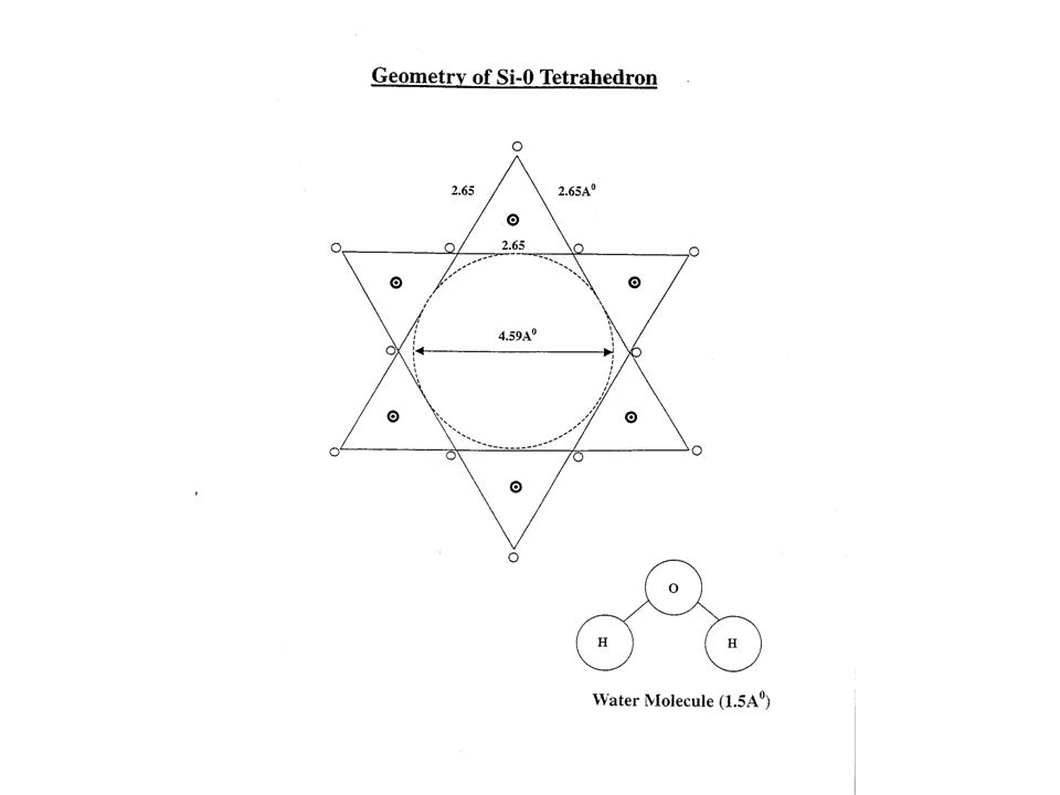
13. Role of Water Vapor Small molecule (< 3 A o ) Easily fits the cavity of 6-member SiO 2 tetrahedra Need only few molecules of H 2 O Hence fatigue can occur at low RH Higher the humidity, higher the fatigue No fatigue in vacuum

14. Role of Stress Stress is the catalyst Higher the stress, higher the fatigue

15. Role of Temperature Vibrational energy of H 2 O molecule vs. T Chemical reaction of SiO 2 with H 2 O vs. T Vibrational energy of glass forming oxides,SiO 2, Na 2 O, CaO, B 2 O 3, etc. vs. T Fatigue vs. Coeff. Thermal Expansion Fatigue at subzero temperature

16. Role of Stress Duration (SiO 2 + H 2 O + stress) reaction requires time Short duration of time means less fatigue Long duration of stress means more fatigue

17. Measurement of Strength 4-point Bend Test (uniaxial) Tensile Test(uniaxial) Ring-on-Ring Test (biaxial) ASTM Standard Test Duration Test Environment

18. St. Venant Flexure M/I = E/R =  /y MOR =  f = 1.5 P (L – l ) / (b t 2 ) P = load at failure L = support span l = load span b = width of specimen t = thickness of specimen

19. Strength Distribution Gaussian Weibull P f = 1 – exp [ - (  /  o ) m ] P f : failure probability at stress   o : stress at P f = 0.63 m : slope of (lnlnP f vs. ln  )

20. Weibull Distribution Unimodal (single value of m, i.e. uniform flaw) Multimodal (multiple values of m, i.e. multiple families of flaw) Physical meaning of m: approx.(mean  f / std.dev) Fatigue is difficult to measure for multiple families of flaw

21. Measurement of Dynamic Fatigue d  /dt (MPa/s) N   (MPa) mt (s) 3.020751525 0.3206818250 0.032059162500 0.0320451925000 0.003203017250000

22. Weibull Distribution Plot Weibullized Eagle SG dynamic fatigue at each rate, fastest rate (#1) has the strongest distribution.

23. Computation of Fatigue Constant Let   = median strength at (d  /dt) 1 Let    = median strength at (d  /dt) 2 Then  1 /  2 = [ (d  /dt) 1 / (d  /dt) 2 ] 1/(n + 1)

24. ln  vs. ln (d  dt) Plot 1 n+1

26. Dynamic Fatigue Constants for Silicate Glasses (ambient environment) Glass CodeCompositionAvg. n Value CTE (25-300C) 9061CTV Panel1498 0080SLS1680 7740Pyrex2732 7059 Color Filter 2838 1737LCD2437 1723SAS3036 7940FS375.5 7971ULE450.3

27. Plot of n vs. CTE

28. Physical Meaning of n n Value Strength loss due to 10X lower (d  / dt) 1513.4 % 2010.4 % 258.5 % 307.2 % 356.2 % 405.5 %

29. Measurement of Static fatigue Apply static (constant) stress  to 4-point bend specimen and measure time t f till it fails Plot ln  vs. t f Estimate n value from  1 n t f1 =  2 n t f2 n = [ (ln t f2 – ln t f1 ) / (ln  1 – ln  2 ) ]

30. Plot of ln  vs. ln t f ** * *** * *** *** ln (time) ln(stress) * * ** 1/n 1

32. Comparison of Static vs. Dynamic n Values Dynamic n > Static n Code 9061 glass: n d = 22, n s = 14 CO diesel filter: n d = 30, n s = 15

33. Allowance for Fatigue Damage ( LD Diesel Filter ) Recall  n t f = constant New Filter:  1 =  o, t f = t o = 1 sec. AT Filter for LDD application: n = 70, Life = 200,000 Km Regen. Freq’y: 300 Km  max Duration: 75 sec. each regen. Find fatigue factor & usable strength

34. LD Diesel Filter (cont’d) Total regens = 200,000 Km / 300 KM = 667 Total stress duration = 667 x 75 s = 50,000 s. Useable strength =  2 as shown below  2 n x 50,000 =  1 n x 1  2 =  1 [ 1 / 50,000 ] 1/n = 0.86  1 = 0.86  o Fatigue Factor = 0.86

35. Allowance for Fatigue Damage ( HD Diesel Filter ) CO Filter for HDD application n =30, Life = 700,000 Km Regen. Freq’y = 400 Km  max Duration = 100 s Total Regens = 1750 Total Stress Duration = 175,000 s  2 = [ 1/175,000 ] 1/30 = 0.67  o Fatigue Factor = 0.67

36. Allowance for Stressed Area ( HD Diesel Filter ) Assume 9” diameter x 12” long filter Assume m = 15 Area Factor = [ A spec / A filter ] 1/m A spec = 0.75” x 1” = 0.75 in 2 A filter = 3.14 x D x L = 113 in 2 Area Factor = 0.72

37. Allowance for Acceptable P f ( HD Diesel Filter ) Failure Probability Factor = ( P f ) 1/m, m = 15 FPF = 0.54for P f = 0.0001 (0.01 % fail) FPF = 0.46 for P f = 0.00001 (0.001% fail)

38. Final Useable Strength of CO Filter for HD Diesel Filter Useable Strength =  o x FF x AF x FPF = 0.26  o for P f = 0.01% = 0.22  o for P f =0.001%

39. Threshold Stress (fatigue free stress) At certain value of stress, known as threshold stress, the critical flaw does not propagate Materials can sustain threshold stress without becoming weak, hence we may call that “happy stress”

40. Static Fatigue Test for Estimating Threshold Stress Use 4-point bend test at 400C Measure MOR of 15 specimens Assume n =n dyn and estimate allowable stress (  eas ) for 9 x 12 filter at P f = 0.001% Apply static stress =  eas on 15 specimens =  eas + 50 psi on 15 specimens =  eas + 75 psi on 15 specimens Hold above static stresses for 100 hours at 400C Record any premature failures Remove stress Measure MOR of surviving specimens for each set Compare MOR distributions before and after static stress Expect max. loss of strength at highest static stress and none at  eas

41. Static Fatigue Fixture with Multiple Specimens

42. Static Fatigue Fixture in 400C Oven

43. Comparison of Strength Distributions after Static Load Test CO-E1(axial) Static Load then Residual MOR at 400 o C

44. Strength Data for CO 200/12 Baseline:353 psi(  s = 0 ) MOR res :296 psi (  s = 150 psi ) MOR res :243 psi(  s = 175 psi ) MOR res :187 psi (  s = 200 psi )

45. Crack Growth during Static Loading a r / a i = [ MOR i / MOR res ] 2 a r / a i = 1.42 @ 150 psi = 2.11 @ 175 psi = 3.56 @ 200 psi Estimated n value: ~15

46. Static vs. Dynamic n Values Static value is lower than dynamic value due to longer time for stress corrosion reaction in humid environment Which n value should be used? This will depend on stress/time history for a given application

47. Applications of Fatigue Effect Color TV Panel Space Shuttle Windows Fiber Optics Catalytic Converters Diesel Filters LCD Panel

48. Acknowledgements John Helfinstine Janto Widjaja