1. SAS® Global Forum 2014 March 23-26 Washington, DC Got Randomness?
SASTM for Mixed
and Generalized
Linear Mixed Models
David A. Dickey
NC State University
TM SAS and its products are the registered
trademarks of SAS Institute, Cary, NC
Copyright © 2010, SAS Institute Inc. All rights reserved.

2. Data: Challenger
(Binomial with
random effects)
Data: Ships
(Poisson with
offset)
Data: Crab mating patterns (X rated)
(Poisson Regression, ZIP model,
Negative Binomial)
Data: Typists
(Poisson with
random effects)
Data: Flu samples
(Binomial with
random effects)

3. “Generalized”  non normal distribution
Binary for probabilities: Y=0 or 1
Mean E{Y}=p Variance p(1-p)
Pr{Y=j}= pj(1-p)(1-j)
Link: L=ln(p/(1-p)) = “Logit”
Range (over all L): 0<p<1
Poisson for counts: Y in {0,1,2,3,4, ….}
Mean count l Variance l
Pr{Y=j} = exp(- l )(lj)/(j!)
Link: L = log(l)
Range (over all L): l >0
2/3
1/3
Like Dislike
Pr{ Like }=2/3
l=0.4055
2/3
.055
.27
.007
.001

4. Mixed (not generalized) Models: Fixed Effects and Random Effects

5. Fixed? or Random?
Replication : Same levels Different levels
Inference for: Only Observed Population of
Levels Levels
Levels : Picked on Picked at
Purpose Random
Inference on: Means Variances
Example: Only These All Doctors
Drugs All Clinics
Example: Only These All Farms
Fertilizers All Fields

6. Generalized (not mixed) linear models.
Use link L = g(E{Y}), e.g. ln(p/(1-p)) = ln(E{Y}/(1-E{Y})
Assume L is linear model in the inputs with fixed effects.
Estimate model for L, e.g. L=g(E{Y})=bo + b1 X
Use maximum likelihood
Example:
L = *dose
Dose = 10, L=0.8,
p=exp(0.8)/(1+exp(0.8))=
“inverse link” = 0.86

8. Challenger was mission 24 From 23 previous launches we have:
6 O-rings per mission
Y=0 no damage, Y=1 erosion or blowby
p = Pr {Y=1} = f{mission, launch temperature)
Features: Random mission effects
Logistic link for p
proc glimmix data=O_ring;
class mission;
model fail = temp/dist=binomial s;
random mission;
run;
Generalized
Mixed

9. We “hit the boundary” Estimated G matrix is not positive definite.
Covariance Parameter Estimates
Cov Standard
Parm Estimate Error
mission E
Solutions for Fixed Effects
Effect Estimate Error DF t Value Pr > |t|
Intercept
temp
We “hit the boundary”

10. Likelihood

11. Just logistic regression – no mission variance component

12. input fluseasn year t week pos specimens; pct_pos=100*pos/specimens;
Flu Data CDC
Active Flu Virus
Weekly Data % positive
data FLU;
input fluseasn year t week pos specimens;
pct_pos=100*pos/specimens;
logit=log(pct_pos/100/(1+(pct_pos/100)));
label pos = "# positive specimens";
label pct_pos="% positive specimens";
label t = "Week into flu season (first = week 40)";
label week = "Actual week of year";
label fluseasn = "Year flu season started";
Empirical Logit
% positive

13. S(j) = sin(2pjt/52) C(j)=cos(2pjt/52)
(1) GLM all effects fixed
(harmonic main effects
insignificant)
“Sinusoids”
S(j) = sin(2pjt/52) C(j)=cos(2pjt/52)
PROC GLM DATA=FLU;
class fluseasn;
model logit = s1 c1
fluseasn*s1 fluseasn*c1 fluseasn*s2 fluseasn*c2
fluseasn*s3 fluseasn*c3 fluseasn*s4 fluseasn*c4;
output out=out1 p=p;
data out1; set out1; P_hat = exp(p)/(1+exp(p));
label P_hat = "Pr{pos. sample} (est.)"; run;

14. (2) MIXED analysis
on logits
Random harmonics.
Normality assumed
Toeplitz(1)
PROC MIXED DATA=FLU method=ml;
** reduced model;
class fluseasn;
model logit = s1 c1 /outp=outp outpm=outpm ddfm=kr;
random intercept/subject=fluseasn;
random s1 c1/subject=fluseasn type=toep(1);
random s2 c2/subject=fluseasn type=toep(1);
random s3 c3/subject=fluseasn type=toep(1);
random s4 c4/subject=fluseasn type=toep(1); run;

15. (3) GLIMMIX
analysis
Random harmonics.
Binomial assumed
(overdispersed –
lab effects?)
PROC GLIMMIX DATA=FLU; title2 "GLIMMIX Analysis";
class fluseasn;
model pos/specimens = s1 c1 ; * s2 c2 s3 c3 s4 c4;
random intercept/subject=fluseasn;
random s1 c1/subject=fluseasn type=toep(1);
random s2 c2/subject=fluseasn; ** Toep(1) - no converge;
random s3 c3/subject=fluseasn type=toep(1);
random s4 c4/subject=fluseasn type=toep(1);
random _residual_;
covtest glm;
output out=out2 pred(ilink blup)=pblup
pred(ilink noblup)=overall pearson = p_resid; run;

16. pred(ilink blup)=pblup pred(ilink noblup)= overall pearson = p_resid;
output out=out2
pred(ilink blup)=pblup
pred(ilink noblup)= overall
pearson = p_resid;
run;
Pearson Residuals:
Used to check fit when using
default (pseudo-likelihood)
Variance should be near 1
proc means mean var;
var p_resid; run;
Without random _residual_; variance 
With random _residual_; variance 
Fit Statistics
-2 Res Log Pseudo-Likelihood
Generalized Chi-Square
Gener. Chi-Square / DF
Or… use method=quad

17. random _residual_ does not affect the fit (just standard errors)
Type III Tests of Fixed Effects
Num Den
Effect DF DF F Value Pr > F S c
Tests of Covariance Parameters
Based on the Residual Pseudo-Likelihood
Label DF Res Log P-Like ChiSq Pr > ChiSq Note
Independence < MI
MI: P-value based on a mixture of chi-squares
Output due to
covtest glm; 
random _residual_ does not affect
the fit (just standard errors)

18. Could try 2 parameter Beta distribution instead:
PROC GLIMMIX DATA=FLU; title2 "GLIMMIX Analysis";
class fluseasn;
model f = s1 c1 /dist=beta link=logit s;
random intercept/subject=fluseasn;
random s1 c1/subject=fluseasn type=toep(1);
random s2 c2/subject=fluseasn type=toep(1);
random s3 c3/subject=fluseasn type=toep(1);
random s4 c4/subject=fluseasn type=toep(1);
output out=out3 pred(ilink blup)=pblup
pred(ilink noblup)=overall
pearson=p_residbeta; run;

19. Without BLUPS and with BLUPS
Binomial Assumption
Without BLUPS and with BLUPS

20. Without BLUPS and with BLUPS
Beta Assumption
Without BLUPS and with BLUPS

21. Poisson Example: Wave induced damage
incidents in 40 ships (ship groups)
Variables:
Factorial Effects (fixed, classificatory):
Ship Type levels A,B,C,D,E
Year Constructed levels
Years of Operation levels
Covariate (“offset” - continuous) =
Time in service (“Aggregate months”)
Incidents (dependent, counts)
Source” McCullough & Nelder
(but I ignore cases where year
constructed > period of operation)
Constructed
Operated
60-64
65-69
70-74
75-79
60-74
ABCDE
-X-

22. proc glimmix data=ships;
Title "Ignoring Ship Variance";
class operation construct shiptype;
model incidents = operation construct shiptype/
dist=poisson s offset=log_service; run;
ln(service)
Poisson: ln(l) – ln(service) = b0 + b1(operation) + b2(construct) + b3(ship_type)
ln(l/service)
>1
Ship variance?
-2 Log Likelihood
(more fit statistics)
Pearson Chi-Square
Pearson Chi-Square / DF

23. Without ship variance component:
Type III Tests of Fixed Effects
Num Den
Effect DF DF F Value Pr > F
Operation
Construct
Shiptype

24. PROC GLIMMIX data=ships method=quad;
class operation construct shiptype ship;
model incidents = operation construct shiptype/
dist=poisson s offset=log_service;
covtest "no ship effect" glm;
* random ship;
random intercept / subject = operation*construct*shiptype;
run;
Covariance Parameter Estimates
Standard
Cov Parm Subject Estimate Error
Intercept Operat*Constr*Shipty

25. Fit Statistics
-2 Log Likelihood
Fit Statistics for Conditional Distribution
-2 log L(incidents | r. effects)
Pearson Chi-Square
Pearson Chi-Square / DF
Type III Tests of Fixed Effects
Num Den
Effect DF DF F Value Pr > F
Operation no
Construct 
shiptype changes
Tests of Covariance Parameters  covtest "no ship effect" glm;
Based on the Likelihood
Label DF Log Like ChiSq Pr > ChiSq Note
no ship effect MI
MI: P-value based on a mixture of chi-squares.

26. (reference: SAS GLIMMIX course notes):
Horseshoe Crab study
(reference: SAS GLIMMIX course notes):
Female nests have “satellite” males
Count data – Poisson? Generalized Linear
Features (predictors):
Carapace Width, Weight, Color, Spine condition
Random Effect: Site Mixed Model
To nest 
Go State

27. proc glimmix data=crab; class site; model satellites = weight width /
Fit Statistics
Gener. Chi-Square / DF 2.77
Cov Parm Subject Estimate
Intercept site
Effect Estimate Pr > |t|
Intercept
weight
width
proc glimmix data=crab;
class site;
model satellites = weight width /
dist=poi solution ddfm=kr;
random int / subject=site;
output out=overdisp pearson=pearson; run;
proc means data=overdisp n mean var;
var pearson; run;
proc univariate data=crab normal plot;
var satellites; run;
Histogram # Boxplot
15.5+* .* .
12.5+* |
.* |
.** |
9.5+** |
.*** |
.** |
6.5+******* |
.********
.********** | |
3.5+********** | |
.***** *--+--*
.******** | |
0.5+*******************************
* may represent up to 2 counts
N Mean Variance
Zero Inflated ?

28. Zero Inflated Poisson (ZIP)
Q: Can zero inflation cause overdispersion (s2>m)?
Recall: in Poisson, s2=m=l

29. A: yes!

30. Zero Inflated Poisson - (ZIP code  )
Dickey
ncsu
Zero Inflated Poisson - (ZIP code  )
SAS Global Forum
Washington DC
20745
proc nlmixed data=crab;
parms b0=0 bwidth=0 bweight=0 c0=-2 c1=0 s2u1=1 s2u2=1;
x=c0+c1*width+u1; p0 = exp(x)/(1+exp(x)); * width affects p0;
eta= b0+bwidth*width +bweight*weight +u2;
lambda=exp(eta);
if satellites=0 then
loglike = log(p0 +(1-p0)*exp(-lambda));
else loglike =
log(1-p0)+satellites*log(lambda)-lambda-lgamma(satellites+1);
expected=(1-p0)*lambda; id p0 expected lambda;
model satellites~general(loglike);
Random U1 U2~N([0,0],[s2u1,0,s2u2]) subject=site;
predict p0+(1-p0)*exp(-lambda) out=out1; run;

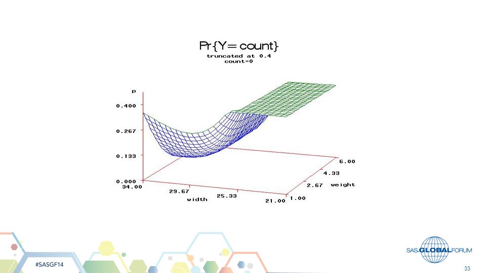
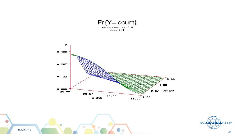
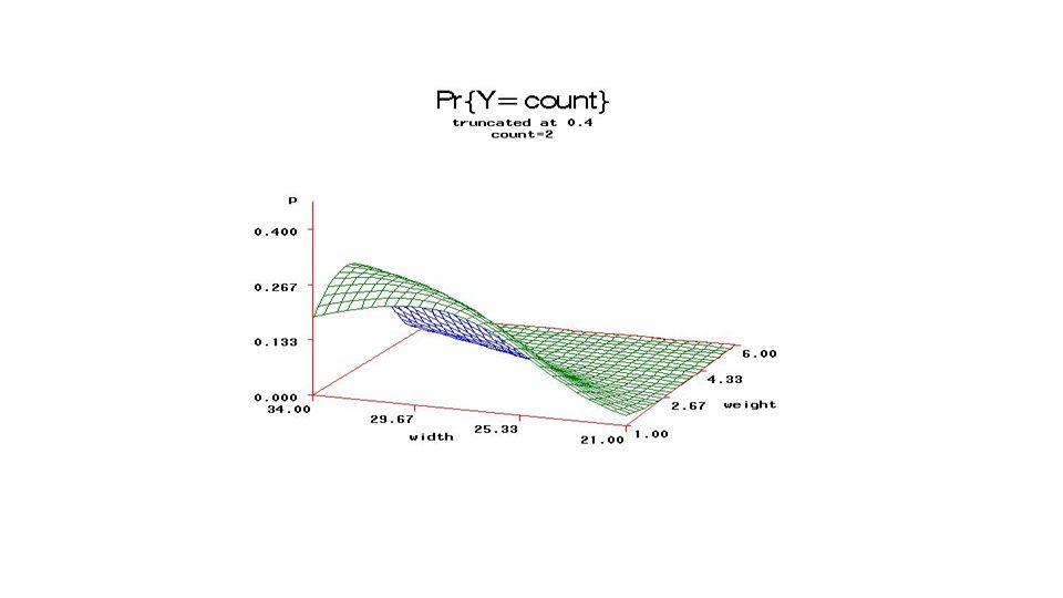
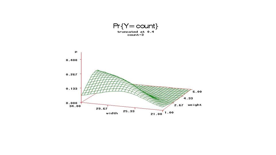
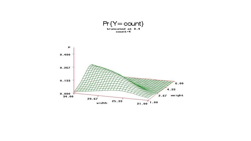
31. weight affects l width affects p0 Parameter Estimates
Parameter Estimate t Pr>|t| Lower Upper b
bwidth
bweight c c
s2u
s2u
weight
affects l
width
affects p0
Variance
for p0 l

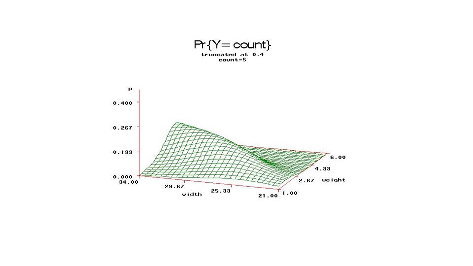
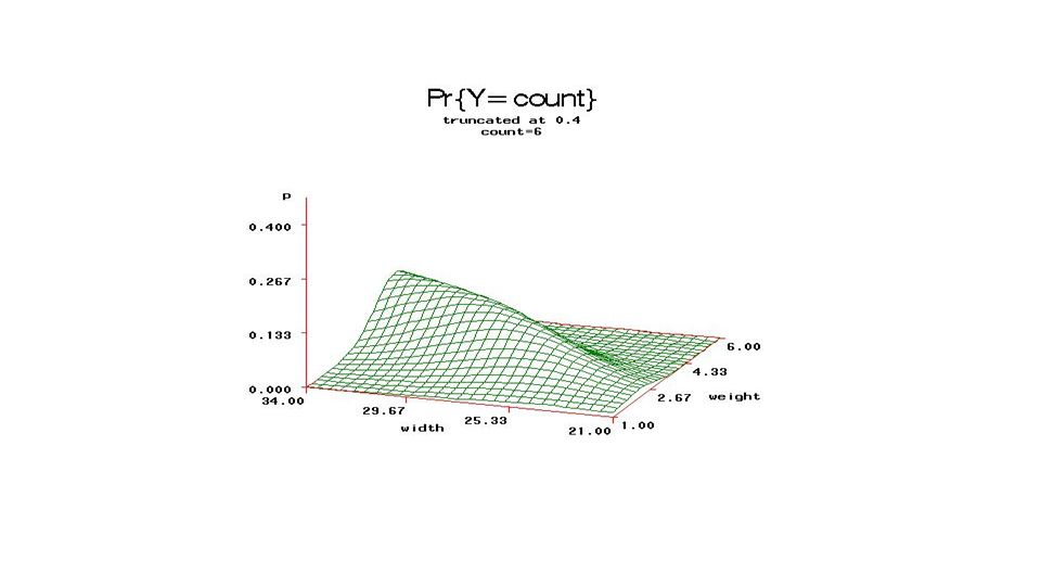
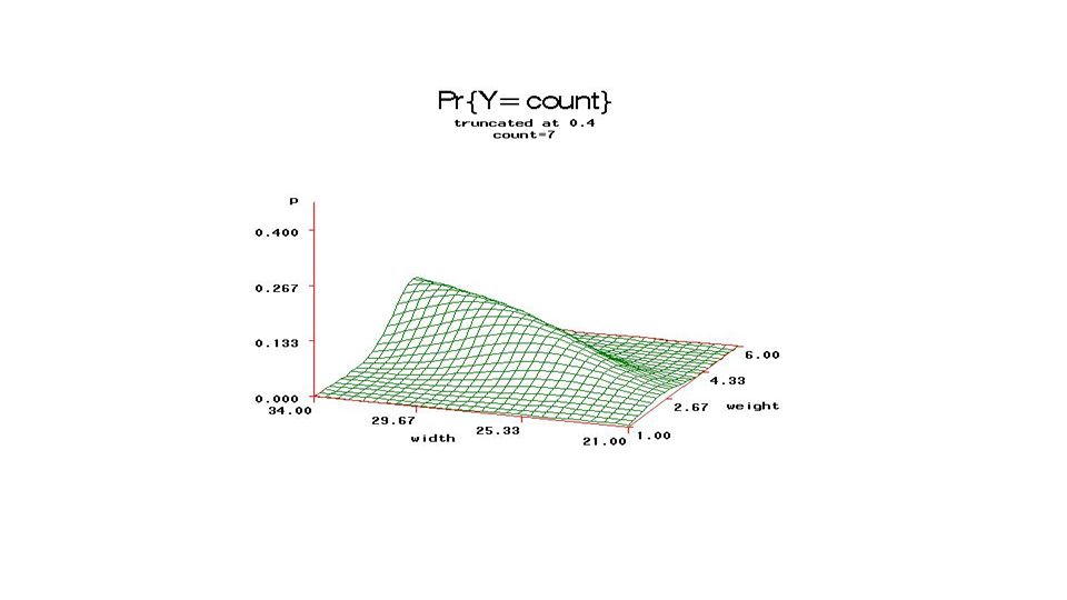
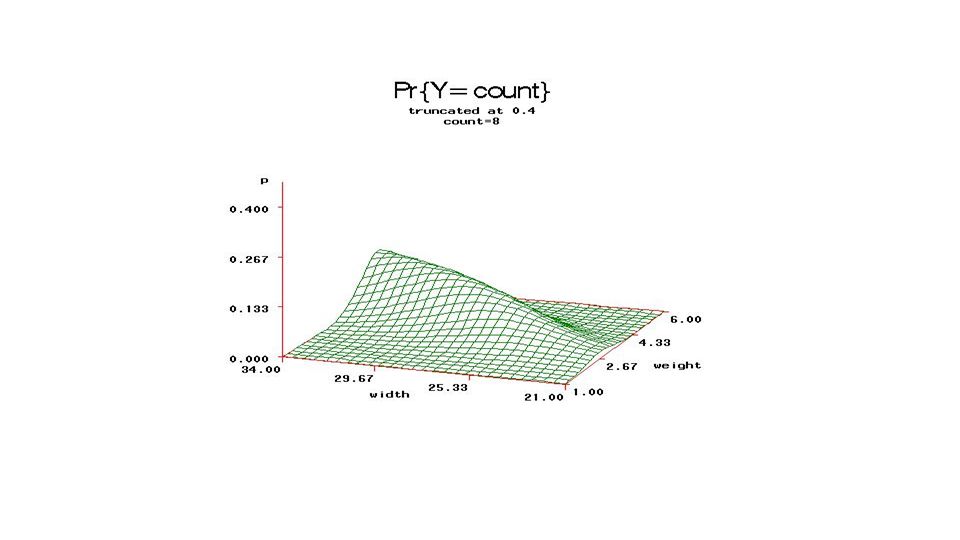
32. From fixed part of model, compute
Pr{count=j} and plot (3D) versus
Weight, Carapace width

42. Another possibility: Negative binomial
Number of failures until kth success ( p=Prob{success} )

43. Negative binomial: In SAS, k (scale) is our 1/k
proc glimmix data=crab; class site;
model satellites = weight width / dist=nb solution ddfm=kr;
random int / subject=site; run;
Fit Statistics
-2 Res Log Pseudo-Likelihood
Generalized Chi-Square
Gener. Chi-Square / DF
Covariance Parameter Estimates
Cov Parm Subject Estimate Std. Error
Intercept site
Scale
Standard
Effect Estimate Error DF t Value Pr > |t|
Intercept
weight
width

44. Population average model vs. Individual Specific Model
8 typists
Y=Error counts (Poisson distributed)
ln(li)= ln(mean of Poisson) = m+Ui for typist i so li=em+Ui
conditionally (individual specific)
Distributions for Y, U~N(0,1) and m=1
l=em=e1=2.7183
= mean for
“typical” typist
(typist with U=0)

45. Population average model
Expectation ||||| | | of individual distributions averaged
across population of all typists.
Run same simulation for 8000 typists, compute mean
of conditional population means, exp(m+U).
The MEANS Procedure
Variable N Mean Std Dev Std Error
ƒƒƒƒƒƒƒƒƒƒƒƒƒƒƒƒƒƒƒƒƒƒƒƒƒƒƒƒƒƒƒƒƒƒƒƒƒƒƒƒƒƒƒƒƒƒ
lambda
Z=( )/ = !!
Population mean is not em
Conditional means, m+U, are lognormal.
Log(Y)~N(1,1) 
E{Y}=exp(m+0.5s2) = e1.5 =
#SASGF13
Copyright © 2013, SAS Institute Inc. All rights reserved.

46. Main points:
Generalized linear models with random effects are subject specific models.
Subject specific models have fixed effects that represent an individual with random effects 0 (individual at the random effect distributional means).
Subject specific models when averaged over the subjects do not give the model fixed effects.
Models with only fixed effects do give the fixed effect part of the model when averaged over subjects and are thus called population average models.