Download presentation
Presentation is loading. Please wait.

1
1 of 14 1/34 Embedded Systems Design: Optimization Challenges Paul Pop Embedded Systems Lab (ESLAB) Linköping University, Sweden
 Linköping University, Sweden")
2
2 of 14 2/34 Outline Embedded systems Example area: automotive electronics Embedded systems design Optimization problems Fault-tolerant mapping and scheduling Voltage scaling Communication delay analysis Assessment and message

3
3 of 14 3/34 Embedded Systems General purpose systemsEmbedded systems Microprocessor market shares

4
4 of 14 4/34 Example Area: Automotive Electronics What is “automotive electronics”? Vehicle functions implemented with electronics Body electronics System electronics: chassis, engine Information/entertainment

5
5 of 14 5/34 Automotive Electronics Market Size 8.9 Market ($billions) 10.513.114.115.817.419.321.0 0 200 400 600 800 1000 1200 1400 19981999200020012002200320042005 Cost of Electronics / Car ($) 90% of future innovations in vehicles: based on electronic embedded systems 2006: 25% of the total cost of a car will be electronics
 Cost of Electronics / Car ($) 90% of future innovations in vehicles: based on electronic embedded systems 2006: 25% of the total cost of a car will be electronics")
6
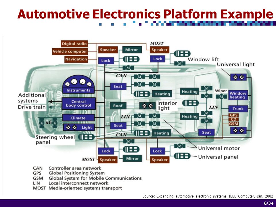
6 of 14 6/34 Automotive Electronics Platform Example Source: Expanding automotive electronic systems, IEEE Computer, Jan. 2002
7
7 of 14 7/34 Outline Embedded systems Example area: automotive electronics Embedded systems design Optimization problems Fault-tolerant mapping and scheduling Voltage scaling Communication delay analysis Assessment and message

8
8 of 14 8/34 Embedded Systems Design Model of system implementation Estimation: exec. time System platform System model System-level design tasks Analysis Software synthesis Hardware synthesis Growing complexity Constraints Time, energy, size Cost, time-to-market Safety, reliability Heterogeneous Hardware components Comm. protocols Mapping and scheduling Voltage scaling Communication delay analysis

9
9 of 14 9/34 Embedded System Design, Cont. Goal: automated design optimization techniques Successfully manage the complexity of embedded systems Meet the constraints imposed by the application domain Shorten the time-to-market Reduce development and manufacturing costs Optimization: the key to successful design

10
10 of 14 10/34 Outline Embedded systems Example area: automotive electronics Embedded systems design Optimization problems Fault-tolerant mapping and scheduling Voltage scaling Communication delay analysis Assessment and message

11
11 of 14 11/34 Optimization Problems 1.Mapping and scheduling 1.1 Mapping to minimize communication 1.2 Mapping and scheduling 1.3 Fault-tolerant mapping and scheduling 2.Voltage scaling 2.1 Continuous voltage scaling 2.2 Discrete voltage scaling 3.Communication delay analysis

12
12 of 14 12/34 Given Application: set of interacting processes Platform: set of nodes Problem #1.1: Mapping P1P1 P4P4 P2P2 P3P3 m1m1 m2m2 m3m3 m4m4 Assessment Optimal solutions even for large problem sizes N1N1 N2N2 P1P1 P4P4 P2P2 P3P3 m1m1 m2m2 m3m3 m4m4 Determine Mapping of processes to nodes Such that the communication is minimized

13
13 of 14 13/34 Problem #1.2: Mapping and Scheduling Given Application: set of interacting processes Platform: set of nodes Timing constraints: deadlines Determine Mapping of processes and messages Schedule tables for processes and messages Such that the timing constraints are satisfied S2S2 S1S1 P1P1 P4P4 P2P2 m1m1 m2m2 m3m3 m4m4 P3P3 N1N1 N2N2 Bus Schedule table Deadline P1P1 P4P4 P2P2 P3P3 m1m1 m2m2 m3m3 m4m4 N1N1 N2N2

14
14 of 14 14/34 Problem #1.2: Assessment Scheduling is NP-complete even in simpler context D. Ullman, “NP-Complete Scheduling Problems”, Journal of Computer Systems Science, volume 10, pages 384–393, 1975. ILP formulation Can’t obtain optimal solutions for large problem sizes Alternative: divide the problem Scheduling Heuristic: List scheduling Mapping Simulated annealing Tabu-search Problem-specific greedy algorithms

15
15 of 14 15/34 Messages: Schedule tables Messages: Fault-tolerant protocol Processes: Schedule tables Fault-Tolerant Mapping and Scheduling... Transient faults TDMA bus: TTP Processes: Re-execution and replication

16
16 of 14 16/34 Fault-Tolerance Techniques P1P1 P1P1 P1P1 Re-execution N1N1 P1P1 P1P1 P1P1 Replication N1N1 N2N2 N3N3 P1P1 P1P1 N1N1 N2N2 P1P1 Re-executed replicas 2

17
17 of 14 17/34 Problem #1.3: Formulation Application: set of process graphsArchitecture: time-triggered system Fault-model: transient faults Given Application: set of interacting processes Platform: set of nodes Timing constraints: deadlines Fault model: number of transient faults in the system period Determine Mapping of processes and messages Schedule tables for processes and messages Fault-tolerance policy assignment Such that the timing constraints are satisfied

18
18 of 14 18/34 P1P1 N1N1 N2N2 TTP P2P2 P3P3 S1S1 S2S2 P4P4 m2m2 Missed Fault-Tolerance Policy Assignment P1P1 P2P2 P3P3 N1N1 N2N2 4050 60 80 P4P4 4050 1 N1N1 N2N2 P1P1 P4P4 P2P2 P3P3 m1m1 m2m2 m3m3 P1P1 N1N1 N2N2 TTP P2P2 P3P3 S1S1 S2S2 m2m2 P4P4 N1N1 N2N2 P1P1 P3P3 S1S1 S2S2 P4P4 P2P2 P1P1 m1m1 m1m1 m2m2 m2m2 P2P2 m3m3 m3m3 P3P3 P4P4 Missed P1P1 N1N1 N2N2 TTP P2P2 P3P3 S1S1 S2S2 m2m2 P4P4 No fault-tolerance: application crashes N1N1 N2N2 P1P1 P3P3 S1S1 S2S2 P4P4 P2P2 P1P1 m2m2 m1m1 TTP Met Optimization of fault-tolerance policy assignment Deadline

19
19 of 14 19/34 Tabu-Search: Policy Assignment & Mapping P1P1 P2P2 P3P3 N1N1 N2N2 4050 60 75 P4P4 4050 1 N1N1 N2N2 P1P1 P4P4 P2P2 P3P3 m1m1 m2m2 m3m3 Design transformations

20
20 of 14 20/34 Problem #2: Voltage Scaling GSM Phone: Search Radio link control Talking MP3 Player Digital Camera: Take photo Restore photo Timing constraints 0 10 20 30 40 50 60 70 199719992002200520082011 Battery power Chip power Power constraints

21
21 of 14 21/34 Problem #2: Voltage Scaling deadline t P 11 22 33 Energy/speed trade-offs: varying the voltages V bs CPU V dd f1f1 f2f2 f3f3 Different voltages: different frequencies Mapping and scheduling: given (fastest freq.) Power deadline t 11 22 33 Slack
 Power deadline t 11 22 33 Slack")
22
22 of 14 22/34 00 22 33 55 44 11 CPU1 CPU2 CPU3 Bus V dd V bs V dd V bs V dd V bs Problem #2.1: Continuous Voltage Scaling Given Application: set of interacting processes Platform: set of nodes, each having supply voltage (V dd ) and body bias voltage (V bs ) inputs Mapping and schedule table (including timing constraints) P deadline t 11 22 33 Slack Architecture and mapping Schedule table / processor
 and body bias voltage (V bs ) inputs Mapping and schedule table (including timing constraints) P deadline t 11 22 33 Slack Architecture and mapping Schedule table / processor")
23
23 of 14 23/34 Problem #2.1: Continuous Voltage Scaling Determine Voltage levels V dd and V bs for each process Such that system energy is minimized and Deadlines are satisfied deadline t P 11 22 33 P t 11 22 33 Slack Output Input Height: voltage level Area: energy Assessment Convex nonlinear problem Polynomial time solvable with an arbitrary good precision A. Andrei, “Overhead-Conscious Voltage Selection for Dynamic and Leakage Energy Reduction of Time-Constrained Systems”, technical report, Linköping University, 2004

24
24 of 14 24/34 Problem #2.1: Formulation Minimize energy E[ 0 ] + E[ 1 ] + E[ 2 ] + E_OH[ 1 - 2 ] Such that T start [ 0 ] + T exe [ 0 ] T start [ 1 ] T start [ 1 ] + T exe [ 1 ] + T oh [ 1 - 2 ] T start [ 2 ] T start [ 2 ] + T exe [ 2 ] DL[ 2 ] Energy due to processes Overhead due to voltage changes Precedence relationships Deadlines
![24 of 14 24/34 Problem #2.1: Formulation Minimize energy E[ 0 ] + E[ 1 ] + E[ 2 ] + E_OH[ 1 - 2 ] Such that T start [ 0 ] + T exe [ 0 ] T start [ 1 ] T start [ 1 ] + T exe [ 1 ] + T oh [ 1 - 2 ] T start [ 2 ] T start [ 2 ] + T exe [ 2 ] DL[ 2 ] Energy due to processes Overhead due to voltage changes Precedence relationships Deadlines](http://images.slideplayer.com/27/9217496/slides/slide_24.jpg "24 of 14 24/34 Problem #2.1: Formulation Minimize energy E[ 0 ] + E[ 1 ] + E[ 2 ] + E_OH[ 1 - 2 ] Such that T start [ 0 ] + T exe [ 0 ] T start [ 1 ] T start [ 1 ] + T exe [ 1 ] + T oh [ 1 - 2 ] T start [ 2 ] T start [ 2 ] + T exe [ 2 ] DL[ 2 ] Energy due to processes Overhead due to voltage changes Precedence relationships Deadlines")
25
25 of 14 25/34 Problem #2.2: Discrete Voltage Scaling Problem formulation Given discrete execution frequencies Processors can operate using a frequency from a fixed discrete set Changing the frequency incurs a delay and an energy penalty Determine the set of frequencies for each task Such that system energy is minimized and Deadlines are satisfied t P deadline 22 33 11 f2f2 f2f2 f2f2 f3f3 f3f3 f1f1 Discrete

26
26 of 14 26/34 Given 1 processor: f {50, 100, 150} MHz 3 processes 1: P={10, 20, 30} mW, dl=1ms, NC=100 cycles 2: P={12, 22, 32} mW, dl=1.5ms, NC=100 cycles 3: P={15, 25, 35} mW, dl=2ms, NC=100 cycles Schedule: execution order is 1, 2, 3 Determine For each process, number of clock cycles to be executed at each frequency such that the energy is minimized Problem #2.2: Example

27
27 of 14 27/34 Problem #2.2: Example, Cont. Assessment: Strongly NP-hard problem The frequencies are now a set of integers; identical to: P. De, “Complexity of the Discrete Time-Cost Tradeoff Problem for Project Networks”, Operations Research, 45(2):302–306, March 1997. Each task has to execute the given number of cycles Task execution time Precedence constraints Deadline constraints Minimize energy MILP formulation for the optimal solution
:302–306, March Each task has to execute the given number of cycles Task execution time Precedence constraints Deadline constraints Minimize energy MILP formulation for the optimal solution.")
28
28 of 14 28/34 Embedded Systems Design Mapped and scheduled model Estimation: exec. time System platform System model System-level design tasks Analysis Software synthesis Hardware synthesis Communication protocols Communication delay analysis

29
29 of 14 29/34 Problem #3: FlexRay Analysis FlexRay communication protocol Becoming de-facto standard in automotive electronics BMW, DaimlerChrysler, General Motors, Volkswagen, Bosch, Motorola, Philips Deterministic data transmission, fault-tolerant, high data-rate... Communication protocol: FlexRay SR Worst-case communication delay Problem Given Application: set of interacting processes Platform: set of nodes connected by FlexRay Implementation: Mapping and scheduling Determine Worst-case communication delays for messages

30
30 of 14 30/34 Problem #3: FlexRay Analysis, Cont. StaticDynamicStaticDynamic Generalized Time-division multiple access Flexible Time-division multiple access Bus cycle m4m4 m5m5 m6m6 m7m7 Arrive dynamically Off-line: Worst- case analysis Off-line: Schedule table m2m2 m3m3 m1m1 Statically assigned

31
31 of 14 31/34 Problem #3: Formulation and Example Given FlexRay bus Length of the static phase Length of the dynamic phase Dynamically arriving messages Priorities Determine for each message Worst-case communication delay Static Dynamic Fixed size bin m4m4 m5m5 m6m6 m7m7 Priority Dynamic Analyze this! m4m4 m5m5 m6m6 m7m7 Static Bin covering: two bins

32
32 of 14 32/34 Problem #3: Assessment ”Classic” bin covering problem Given Set of bins of fixed integer size Set of items of integer size Determine Maximum number of bins that can be filled with the items Assessment Asymptotic fully polynomial time approximation FlexRay dynamic phase analysis ≠ ”classic” bin covering Bins have an upper limit: size of the dynamic phase Assessment Approximation algorithm does not exist MILP formulation feasible up to 60 messages Wanted: better solution

33
33 of 14 33/34 Outline Embedded systems Example area: automotive electronics Embedded systems design Optimization problems Fault-tolerant mapping and scheduling Voltage scaling Communication delay analysis Assessment and message

34
34 of 14 34/34 Message Optimization Key to successful embedded systems design Challenges Classify the problems Divide the problem into sub-problems Formulate the problems Solve the problems optimally Fast and accurate heuristics for specific problems

Similar presentations


