1. 6.1 - One Sample 6.1 - One Sample  Mean μ, Variance σ 2, Proportion π 6.2 - Two Samples 6.2 - Two Samples  Means, Variances, Proportions μ 1 vs. μ 2 σ 1 2 vs. σ 2 2 π 1 vs. π 2 μ 1 vs. μ 2 σ 1 2 vs. σ 2 2 π 1 vs. π 2 6.3 - Multiple Samples 6.3 - Multiple Samples  Means, Variances, Proportions μ 1, …, μ k σ 1 2, …, σ k 2 π 1, …, π k μ 1, …, μ k σ 1 2, …, σ k 2 π 1, …, π k CHAPTER 6 Statistical Inference & Hypothesis Testing CHAPTER 6 Statistical Inference & Hypothesis Testing

2. 6.1 - One Sample 6.1 - One Sample  Mean μ, Variance σ 2, Proportion π 6.2 - Two Samples 6.2 - Two Samples  Means, Variances, Proportions μ 1 vs. μ 2 σ 1 2 vs. σ 2 2 π 1 vs. π 2 μ 1 vs. μ 2 σ 1 2 vs. σ 2 2 π 1 vs. π 2 6.3 - Multiple Samples 6.3 - Multiple Samples  Means, Variances, Proportions μ 1, …, μ k σ 1 2, …, σ k 2 π 1, …, π k μ 1, …, μ k σ 1 2, …, σ k 2 π 1, …, π k CHAPTER 6 Statistical Inference & Hypothesis Testing CHAPTER 6 Statistical Inference & Hypothesis Testing

3. Consider two independent populations… Null Hypothesis H 0 : μ 1 = μ 2, i.e., μ 1 – μ 2 = 0 (“No mean difference") Test at signif level α POPULATION 1 and a random variable X, normally distributed in each. POPULATION 2 Classic Example: “Randomized Clinical Trial”… Pop 1 = Treatment, Pop 2 = Control X 2 ~ N( μ 2, σ 2 ) 11 σ1σ1 22 σ2σ2 X 1 ~ N( μ 1, σ 1 ) Random Sample, size n 1 Random Sample, size n 2 Sampling Distribution =?  μ0 μ0

4. Consider two independent populations… Null Hypothesis H 0 : μ 1 = μ 2, i.e., μ 1 – μ 2 = 0 (“No mean difference") Test at signif level α POPULATION 1 and a random variable X, normally distributed in each. POPULATION 2 Classic Example: “Randomized Clinical Trial”… Pop 1 = Treatment, Pop 2 = Control X 2 ~ N( μ 2, σ 2 ) 11 σ1σ1 22 σ2σ2 X 1 ~ N( μ 1, σ 1 ) Random Sample, size n 1 Random Sample, size n 2 Sampling Distribution =?  μ0 μ0

5. Mean(X – Y) = Mean(X) – Mean(Y) Consider two independent populations… Null Hypothesis H 0 : μ 1 = μ 2, i.e., μ 1 – μ 2 = 0 (“No mean difference") Test at signif level α POPULATION 1 and a random variable X, normally distributed in each. POPULATION 2 Classic Example: “Randomized Clinical Trial”… Pop 1 = Treatment, Pop 2 = Control X 2 ~ N( μ 2, σ 2 ) 11 σ1σ1 22 σ2σ2 X 1 ~ N( μ 1, σ 1 ) Random Sample, size n 1 Random Sample, size n 2 Sampling Distribution =? Recall from section 4.1 (Discrete Models): and if X and Y are independent… Var(X – Y) = Var(X) + Var(Y)  μ0 μ0

6. Consider two independent populations… Null Hypothesis H 0 : μ 1 = μ 2, i.e., μ 1 – μ 2 = 0 (“No mean difference") Test at signif level α POPULATION 1 and a random variable X, normally distributed in each. POPULATION 2 Classic Example: “Randomized Clinical Trial”… Pop 1 = Treatment, Pop 2 = Control X 2 ~ N( μ 2, σ 2 ) 11 σ1σ1 22 σ2σ2 X 1 ~ N( μ 1, σ 1 ) Random Sample, size n 1 Random Sample, size n 2 Sampling Distribution =? Recall from section 4.1 (Discrete Models): Mean(X – Y) = Mean(X) – Mean(Y) and if X and Y are independent… Var(X – Y) = Var(X) + Var(Y)  μ0 μ0

7. Consider two independent populations… Null Hypothesis H 0 : μ 1 = μ 2, i.e., μ 1 – μ 2 = 0 (“No mean difference") Test at signif level α POPULATION 1 and a random variable X, normally distributed in each. POPULATION 2 Classic Example: “Randomized Clinical Trial”… Pop 1 = Treatment, Pop 2 = Control X 2 ~ N( μ 2, σ 2 ) 11 σ1σ1 22 σ2σ2 X 1 ~ N( μ 1, σ 1 ) Random Sample, size n 1 Random Sample, size n 2 Sampling Distribution =? Recall from section 4.1 (Discrete Models): Mean(X – Y) = Mean(X) – Mean(Y) and if X and Y are independent… Var(X – Y) = Var(X) + Var(Y)  μ0 μ0

8. Consider two independent populations… Null Hypothesis H 0 : μ 1 = μ 2, i.e., μ 1 – μ 2 = 0 (“No mean difference") Test at signif level α POPULATION 1 and a random variable X, normally distributed in each. POPULATION 2 Classic Example: “Randomized Clinical Trial”… Pop 1 = Treatment, Pop 2 = Control X 2 ~ N( μ 2, σ 2 ) 11 σ1σ1 22 σ2σ2 X 1 ~ N( μ 1, σ 1 ) Random Sample, size n 1 Random Sample, size n 2 Sampling Distribution =? Recall from section 4.1 (Discrete Models): Mean(X – Y) = Mean(X) – Mean(Y) and if X and Y are independent… Var(X – Y) = Var(X) + Var(Y)  μ0 μ0

9. Consider two independent populations… Null Hypothesis H 0 : μ 1 = μ 2, i.e., μ 1 – μ 2 = 0 (“No mean difference") Test at signif level α POPULATION 1 and a random variable X, normally distributed in each. POPULATION 2 Classic Example: “Randomized Clinical Trial”… Pop 1 = Treatment, Pop 2 = Control X 2 ~ N( μ 2, σ 2 ) 11 σ1σ1 22 σ2σ2 X 1 ~ N( μ 1, σ 1 ) Random Sample, size n 1 Random Sample, size n 2 Sampling Distribution =? Recall from section 4.1 (Discrete Models): Mean(X – Y) = Mean(X) – Mean(Y) and if X and Y are independent… Var(X – Y) = Var(X) + Var(Y)  μ0 μ0

10. Consider two independent populations… Null Hypothesis H 0 : μ 1 = μ 2, i.e., μ 1 – μ 2 = 0 (“No mean difference") Test at signif level α POPULATION 1 and a random variable X, normally distributed in each. POPULATION 2 Classic Example: “Randomized Clinical Trial”… Pop 1 = Treatment, Pop 2 = Control X 2 ~ N( μ 2, σ 2 ) 11 σ1σ1 22 σ2σ2 X 1 ~ N( μ 1, σ 1 ) Random Sample, size n 1 Random Sample, size n 2 Sampling Distribution =? Recall from section 4.1 (Discrete Models): Mean(X – Y) = Mean(X) – Mean(Y) and if X and Y are independent… Var(X – Y) = Var(X) + Var(Y)  μ0 μ0

11. Consider two independent populations… Null Hypothesis H 0 : μ 1 = μ 2, i.e., μ 1 – μ 2 = 0 (“No mean difference") Test at signif level α POPULATION 1 and a random variable X, normally distributed in each. POPULATION 2 Classic Example: “Randomized Clinical Trial”… Pop 1 = Treatment, Pop 2 = Control X 2 ~ N( μ 2, σ 2 ) 11 σ1σ1 22 σ2σ2 X 1 ~ N( μ 1, σ 1 ) Random Sample, size n 1 Random Sample, size n 2 Sampling Distribution =? Recall from section 4.1 (Discrete Models): Mean(X – Y) = Mean(X) – Mean(Y) and if X and Y are independent… Var(X – Y) = Var(X) + Var(Y)  μ0 μ0 = 0 under H 0

12. Consider two independent populations… Null Hypothesis H 0 : μ 1 = μ 2, i.e., μ 1 – μ 2 = 0 (“No mean difference") Test at signif level α POPULATION 1 and a random variable X, normally distributed in each. POPULATION 2 X 2 ~ N( μ 2, σ 2 ) 11 σ1σ1 22 σ2σ2 X 1 ~ N( μ 1, σ 1 ) Null Distribution 0 s.e. But what if σ 1 2 and σ 2 2 are unknown? Then use sample estimates s 1 2 and s 2 2 with Z- or t-test, if n 1 and n 2 are large.

13. Consider two independent populations… Null Hypothesis H 0 : μ 1 = μ 2, i.e., μ 1 – μ 2 = 0 (“No mean difference") Test at signif level α POPULATION 1 and a random variable X, normally distributed in each. POPULATION 2 X 2 ~ N( μ 2, σ 2 ) 11 σ1σ1 22 σ2σ2 X 1 ~ N( μ 1, σ 1 ) Null Distribution 0 s.e. But what if σ 1 2 and σ 2 2 are unknown? Then use sample estimates s 1 2 and s 2 2 with Z- or t-test, if n 1 and n 2 are large. (But what if n 1 and n 2 are small?) Later… L a t e r …

14. Example: X = “$ Cost of a certain medical service” Data Sample 1: n 1 = 137 NOTE: > 0 Assume X is known to be normally distributed at each of k = 2 health care facilities (“groups”). Clinic: X 2 ~ N( μ 2, σ 2 )Hospital: X 1 ~ N( μ 1, σ 1 ) Null Hypothesis H 0 : μ 1 = μ 2, i.e., μ 1 – μ 2 = 0 (“No difference exists.") 2-sided test at significance level α =.05 Sample 2: n 2 = 140 Null Distribution 0 4.2 95% Confidence Interval for μ 1 – μ 2 : 95% Margin of Error = (1.96)(4.2) = 8.232 (84 – 8.232, 84 + 8.232) =(75.768, 92.232) does not contain 0 Z-score = = 20 >> 1.96  p <<.05 Reject H 0 ; extremely strong significant difference

15. Null Hypothesis H 0 : μ 1 = μ 2, i.e., μ 1 – μ 2 = 0 (“No mean difference") Test at signif level α POPULATION 1POPULATION 2 X 2 ~ N( μ 2, σ 2 ) 11 22 X 1 ~ N( μ 1, σ 1 ) Null Distribution Sample size n 1 Sample size n 2 Consider two independent populations…and a random variable X, normally distributed in each.  large n 1 and n 2

16. Null Hypothesis H 0 : μ 1 = μ 2, i.e., μ 1 – μ 2 = 0 (“No mean difference") Test at signif level α POPULATION 1POPULATION 2 X 2 ~ N( μ 2, σ 2 ) 11 22 X 1 ~ N( μ 1, σ 1 ) Null Distribution Sample size n 1 Sample size n 2 Consider two independent populations…and a random variable X, normally distributed in each.  large n 1 and n 2  small n 1 and n 2 “pooled” then conduct a t-test on the “pooled” samples. equivariant IF the two populations are equivariant, i.e.,

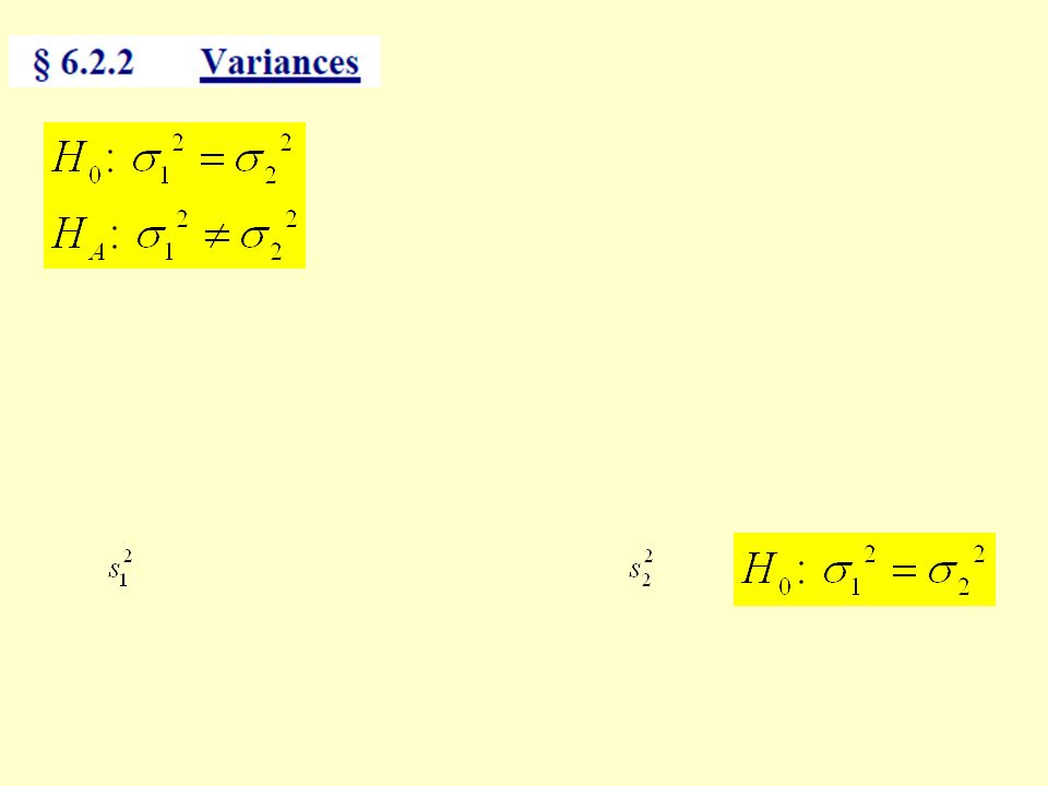
18. Test Statistic Sampling Distribution =? Working Rule of Thumb Acceptance Region for H 0 ¼ < F < 4 Working Rule of Thumb Acceptance Region for H 0 ¼ < F < 4

19. Null Hypothesis H 0 : μ 1 = μ 2, i.e., μ 1 – μ 2 = 0 (“No mean difference") Test at signif level α POPULATION 1POPULATION 2 X 2 ~ N( μ 2, σ 2 ) 11 22 X 1 ~ N( μ 1, σ 1 ) Null Distribution Consider two independent populations…and a random variable X, normally distributed in each.  small n 1 and n 2 “pooled” is accepted, then estimate their common value with a “pooled” sample variance. equal variances IF equal variances The pooled variance is a weighted average of s 1 2 and s 2 2, using the degrees of freedom as the weights.

20. Null Hypothesis H 0 : μ 1 = μ 2, i.e., μ 1 – μ 2 = 0 (“No mean difference") Test at signif level α POPULATION 1POPULATION 2 X 2 ~ N( μ 2, σ 2 ) 11 22 X 1 ~ N( μ 1, σ 1 ) Null Distribution Consider two independent populations…and a random variable X, normally distributed in each.  small n 1 and n 2 “pooled” is accepted, then estimate their common value with a “pooled” sample variance. equal variances IF equal variances The pooled variance is a weighted average of s 1 2 and s 2 2, using the degrees of freedom as the weights. is rejected, equal variances IF equal variances SEE LECTURE NOTES AND TEXTBOOK. then use Satterwaithe Test, Welch Test, etc. SEE LECTURE NOTES AND TEXTBOOK.

21. s 2 = SS/df Example: Y = “$ Cost of a certain medical service” Assume Y is known to be normally distributed at each of k = 2 health care facilities (“groups”). Clinic: Y 2 ~ N( μ 2, σ 2 )Hospital: Y 1 ~ N( μ 1, σ 1 ) Null Hypothesis H 0 : μ 1 = μ 2, i.e., μ 1 – μ 2 = 0 (“No difference exists.") 2-sided test at significance level α =.05 Data: Sample 1 = {667, 653, 614, 612, 604}; n 1 = 5 Sample 2 = { 593, 525, 520}; n 2 = 3 Analysis via T-test (if equivariance holds): Point estimates NOTE: > 0 “Group Means” The pooled variance is a weighted average of the group variances, using the degrees of freedom as the weights. “Group Variances” Pooled Variance SS 1 SS 2 df 1 df 2

22. df = 6 s 2 = SS/df p-value = Example: Y = “$ Cost of a certain medical service” Assume Y is known to be normally distributed at each of k = 2 health care facilities (“groups”). Clinic: Y 2 ~ N( μ 2, σ 2 )Hospital: Y 1 ~ N( μ 1, σ 1 ) Null Hypothesis H 0 : μ 1 = μ 2, i.e., μ 1 – μ 2 = 0 (“No difference exists.") 2-sided test at significance level α =.05 Standard Error > 2 * (1 - pt(3.5, 6)) [1] 0.01282634 Reject H 0 at α =.05 stat signif, Hosp > Clinic Data: Sample 1 = {667, 653, 614, 612, 604}; n 1 = 5 Sample 2 = { 593, 525, 520}; n 2 = 3 Analysis via T-test (if equivariance holds): Point estimates NOTE: > 0 “Group Means” The pooled variance is a weighted average of the group variances, using the degrees of freedom as the weights. “Group Variances” Pooled Variance SS = 6480

23. R code: > y1 = c(667, 653, 614, 612, 604) > y2 = c(593, 525, 520) > > t.test(y1, y2, var.equal = T) Two Sample t-test data: y1 and y2 t = 3.5, df = 6, p-value = 0.01283 alternative hypothesis: true difference in means is not equal to 0 95 percent confidence interval: 25.27412 142.72588 sample estimates: mean of x mean of y 630 546 p-value < α =.05 Reject H 0 at this level. p-value < α =.05 Reject H 0 at this level. The samples provide evidence that the difference between mean costs is (moderately) statistically significant, at the 5% level, with the hospital being higher than the clinic (by an average of $84). Formal Conclusion Interpretation

24. NEXT UP… PAIRED MEANS page 6.2-7, etc.