1. Stat 112 Notes 6 Today: –Chapter 4.1 (Introduction to Multiple Regression)

2. Multiple Regression In multiple regression analysis, we consider more than one explanatory variable, X 1,…,X K. We are interested in the conditional mean of Y given X 1,…,X K, E(Y| X 1,…,X K ). Two motivations for multiple regression: –We can obtain better predictions of Y by using information on X 1,…,X K rather than just X 1. –We can control for lurking variables

3. Automobile Example A team charged with designing a new automobile is concerned about the gas mileage (gallons per 1000 miles on a highway) that can be achieved. The design team is interested in two things: (1) Which characteristics of the design are likely to affect mileage? (2) A new car is planned to have the following characteristics: weight – 4000 lbs, horsepower – 200, length – 200 inches, seating – 5 adults. Predict the new car’s gas mileage. The team has available information about gallons per 1000 miles and four design characteristics (weight, horsepower, length, seating) for a sample of cars made in 2004. Data is in car04.JMP.

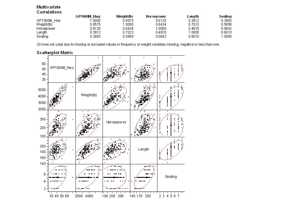
5. Best Single Predictor To obtain the correlation matrix and pairwise scatterplots, click Analyze, Multivariate Methods, Multivariate. If we use simple linear regression with each of the four explanatory variables, which provides the best predictions?

6. Best Single Predictor Answer: The simple linear regression that has the highest R 2 gives the best predictions because recall that Weight gives the best predictions of GPM1000Hwy based on simple linear regression. But we can obtain better predictions by using more than one of the independent variables.

7. Multiple Linear Regression Model

8. Point Estimates for Multiple Linear Regression Model We use the same least squares procedure as for simple linear regression. Our estimates of are the coefficients that minimize the sum of squared prediction errors: Least Squares in JMP: Click Analyze, Fit Model, put dependent variable into Y and add independent variables to the construct model effects box.

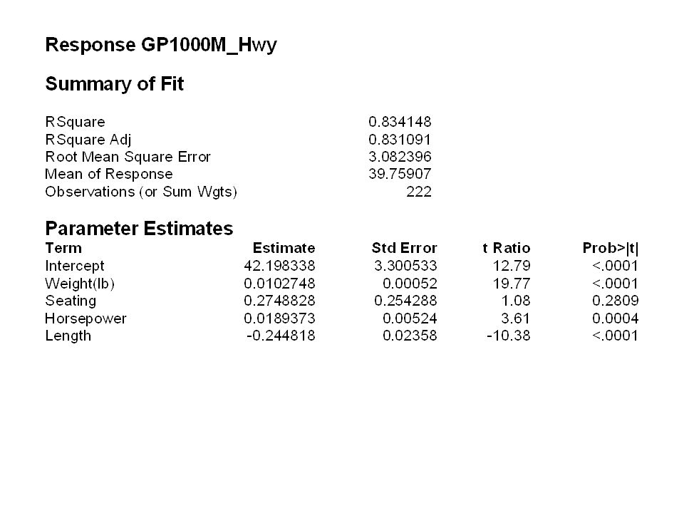
10. Root Mean Square Error Estimate of : = Root Mean Square Error in JMP For simple linear regression of GP1000MHWY on Weight,. For multiple linear regression of GP1000MHWY on weight, horsepower, cargo, seating, The multiple regression improves the predictions.

11. Residuals and Root Mean Square Errors Residual for observation i = prediction error for observation i = Root mean square error = Typical size of absolute value of prediction error As with simple linear regression model, if multiple linear regression model holds –About 95% of the observations will be within two RMSEs of their predicted value For car data, about 95% of the time, the actual GP1000M will be within 2*3.08=6.16 GP1000M of the predicted GP1000M of the car based on the car’s weight, horsepower, length and seating.

12. Residual Example

13. Interpretation of Regression Coefficients Gas mileage regression from car04.JMP