1. How to learn a generative model of images Geoffrey Hinton Canadian Institute for Advanced Research & University of Toronto

2. Each neuron receives inputs from thousands of other neurons –A few neurons also get inputs from the sensory receptors -A few neurons send outputs to muscles. -Neurons use binary spikes of activity to communicate The effect that one neuron has on another is controlled by a synaptic weight – The weights can be positive or negative The synaptic weights adapt so that the whole network learns to perform useful computations –Recognizing objects, understanding language, making plans, controlling the body How the brain works

3. How to make an intelligent system The cortex has about a hundred billion neurons. Each neuron has thousands of connections. So all you need to do is find the right values for the weights on thousands of billions of connections. This task is much too difficult for evolution to solve directly. –A blind search would be much too slow. –DNA doesn’t have enough capacity to store the answer. So there must be an intelligent designer. –What does she look like? –Where did she come from?

4. The intelligent designer The intelligent designer is a learning algorithm. –The algorithm adjusts the weights to give the neural network a better model of the data it encounters. A learning algorithm is the differential equation of knowledge. Evolution produced the learning algorithm –Trial and error in the space of learning algorithms is a much better strategy than trial and error in the space of synapse strengths. To understand the learning algorithm, we first need to understand the type of network it produces. –Shape recognition is a good task to consider. –We are much better than computers and it uses a lot of neurons.

5. Hopfield nets Model each pixel in an image using a binary neuron that has states of 1or 0. Connect the neurons together with symmetric connections. Update the neurons one at a time based on the total input they receive. Stored patterns correspond to the energy minima of the network. 3.7 -4.2 0 0 1 0 1 1 1

6. bias of unit i weight between units i and j Energy of binary configuration s binary state of unit i in configuration s indexes every non-identical pair of i and j once To store a pattern we change the weights to lower the energy of that pattern.

7. Why a Hopfield net doesn’t work The ways in which shapes vary are much too complicated to be captured by pair-wise interactions between pixels. –To capture all the allowable variations of a shape we need extra “hidden” variables that learn to represent the features that the shape is composed of.

8. Some examples of real handwritten digits

9. From Hopfield Nets to Boltzmann Machines Boltzmann machines are stochastic Hopfield nets with hidden variables. They have a simple learning algorithm that adapts all of the interactions so that the equilibrium distribution over the visible variables matches the distribution of the observed data. –The pair-wise interactions with the hidden variables can model higher-order correlations between visible variables.

10. Stochastic binary neurons These have a state of 1 or 0 which is a stochastic function of the neuron’s bias, b, and the input it receives from other neurons. 0.5 0 0 1

11. How a Boltzmann Machine models data The aim of learning is to discover weights that cause the equilibrium distribution of the whole network to match the data distribution on the visible variables. Everything is defined in terms of energies of joint configurations of the visible and hidden units. hidden units visible units

12. The Energy of a joint configuration bias of unit i weight between units i and j Energy with configuration v on the visible units and h on the hidden units binary state of unit i in joint configuration v,h indexes every non-identical pair of i and j once

13. Using energies to define probabilities The probability of a joint configuration over both visible and hidden units depends on the energy of that joint configuration compared with the energy of all other joint configurations. The probability of a configuration of the visible units is the sum of the probabilities of all the joint configurations that contain it. partition function

14. A very surprising fact Everything that one weight needs to know about the other weights and the data in order to do maximum likelihood learning is contained in the difference of two correlations. Derivative of log probability of one training vector Expected value of product of states at thermal equilibrium when the training vector is clamped on the visible units Expected value of product of states at thermal equilibrium when nothing is clamped

15. The batch learning algorithm Positive phase –Clamp a datavector on the visible units. –Let the hidden units reach thermal equilibrium at a temperature of 1 (may use annealing to speed this up) –Sample for all pairs of units –Repeat for all datavectors in the training set. Negative phase –Do not clamp any of the units –Let the whole network reach thermal equilibrium at a temperature of 1 (where do we start?) –Sample for all pairs of units –Repeat many times to get good estimates Weight updates –Update each weight by an amount proportional to the difference in in the two phases.

16. Three reasons why learning is impractical in Boltzmann Machines If there are many hidden layers, it can take a long time to reach thermal equilibrium when a data-vector is clamped on the visible units. It takes even longer to reach thermal equilibrium in the “negative” phase when the visible units are unclamped. –The unconstrained energy surface needs to be highly multimodal to model the data. The learning signal is the difference of two sampled correlations which is very noisy.

17. Restricted Boltzmann Machines We restrict the connectivity to make inference and learning easier. –Only one layer of hidden units. –No connections between hidden units. In an RBM, the hidden units are conditionally independent given the visible states. It only takes one step to reach thermal equilibrium when the visible units are clamped. –So we can quickly get the exact value of : hidden i j visible

18. A picture of the Boltzmann machine learning algorithm for an RBM i j i j i j i j t = 0 t = 1 t = 2 t = infinity Start with a training vector on the visible units. Then alternate between updating all the hidden units in parallel and updating all the visible units in parallel. a fantasy

19. Contrastive divergence learning: A quick way to learn an RBM i j i j t = 0 t = 1 Start with a training vector on the visible units. Update all the hidden units in parallel Update the all the visible units in parallel to get a “reconstruction”. Update the hidden units again. This is not following the gradient of the log likelihood. But it works well. It is trying to make the free energy gradient be zero at the data distribution. reconstruction data

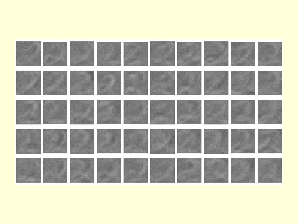
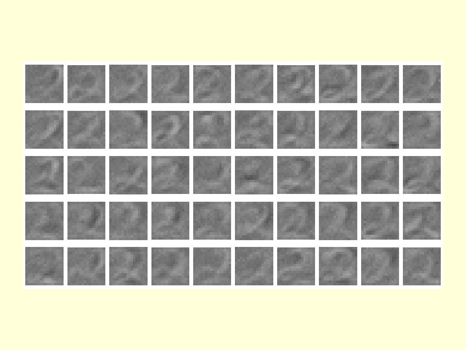
20. How to learn a set of features that are good for reconstructing images of the digit 2 50 binary feature neurons 16 x 16 pixel image 50 binary feature neurons 16 x 16 pixel image Increment weights between an active pixel and an active feature Decrement weights between an active pixel and an active feature data (reality) reconstruction (lower energy than reality) Bush joke

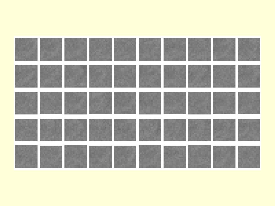
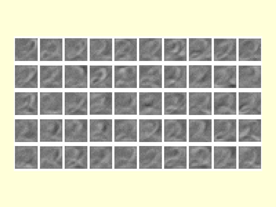
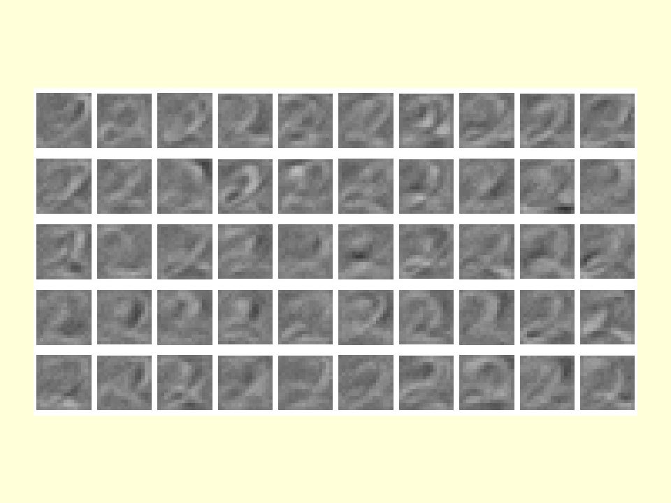
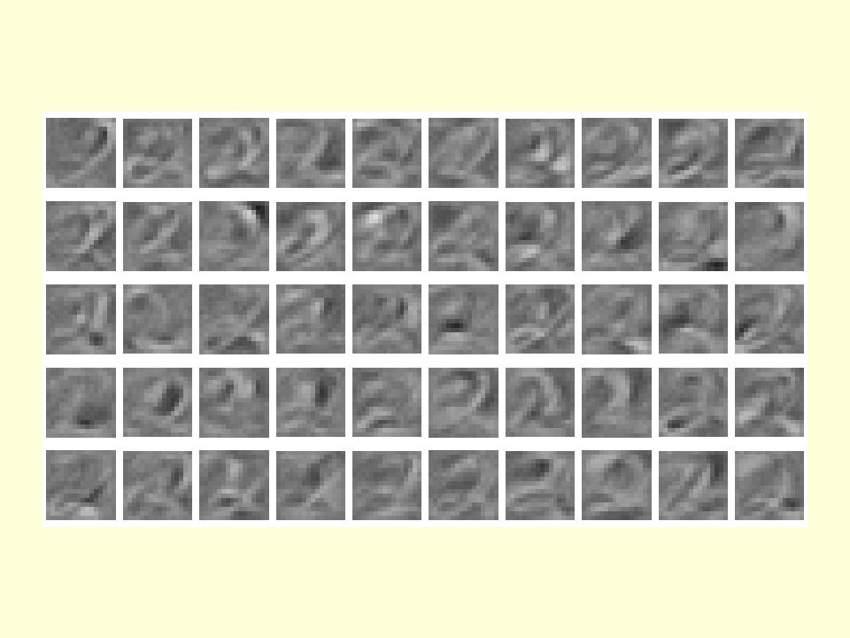
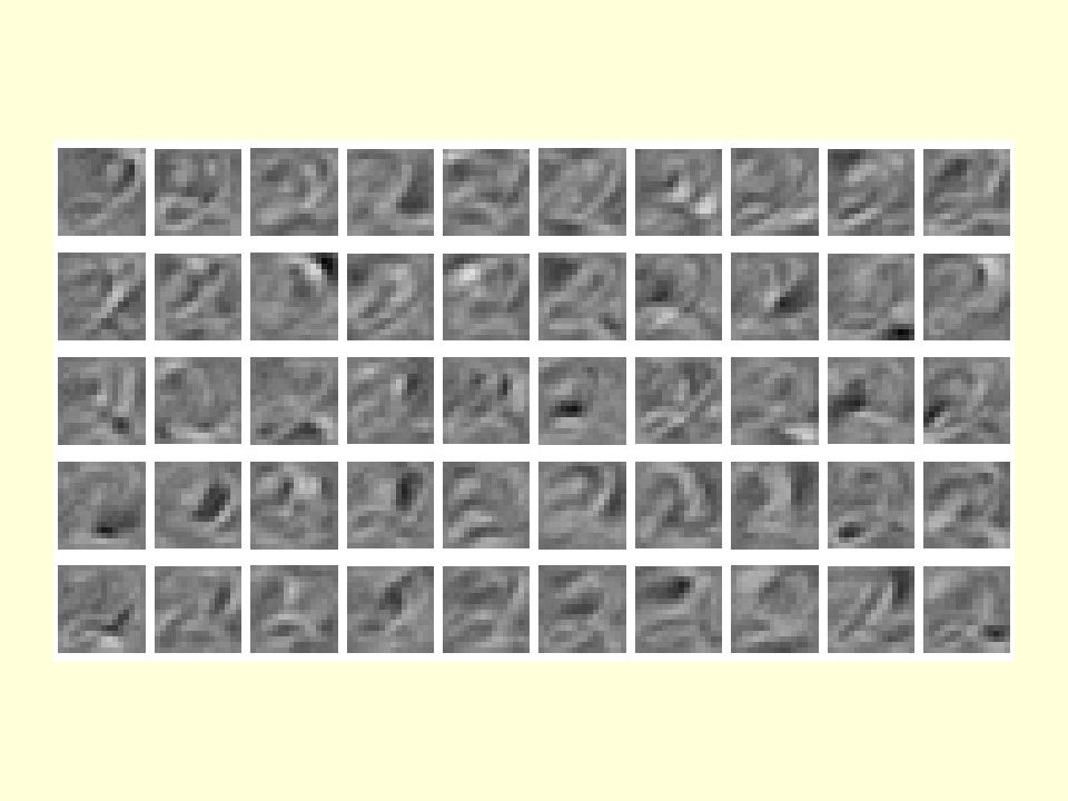
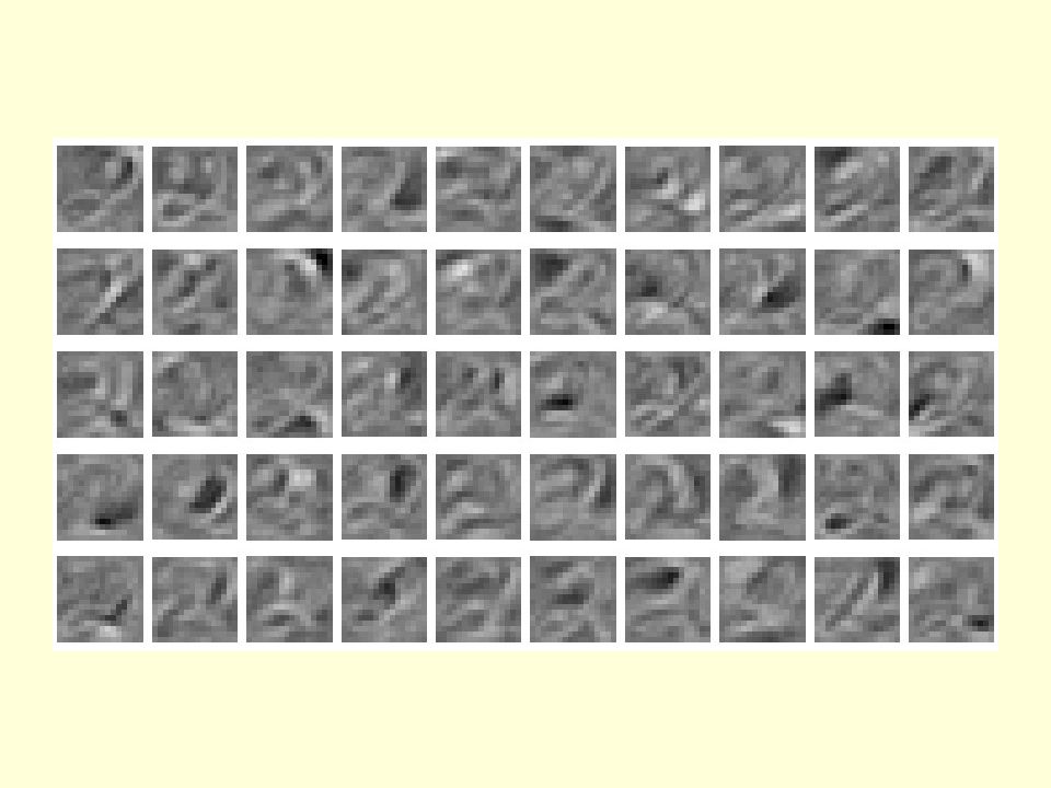
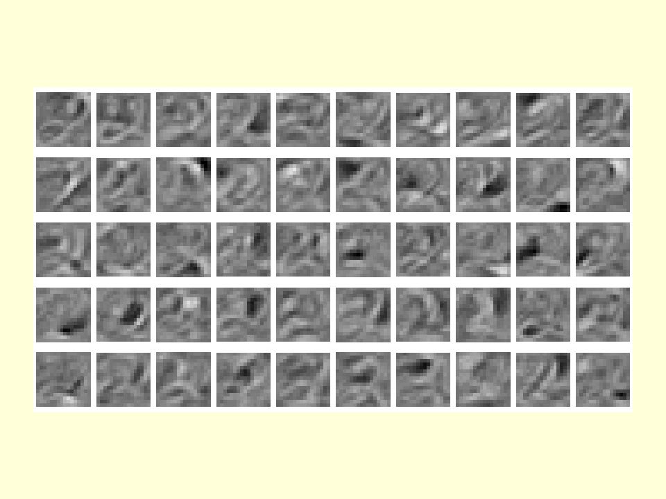
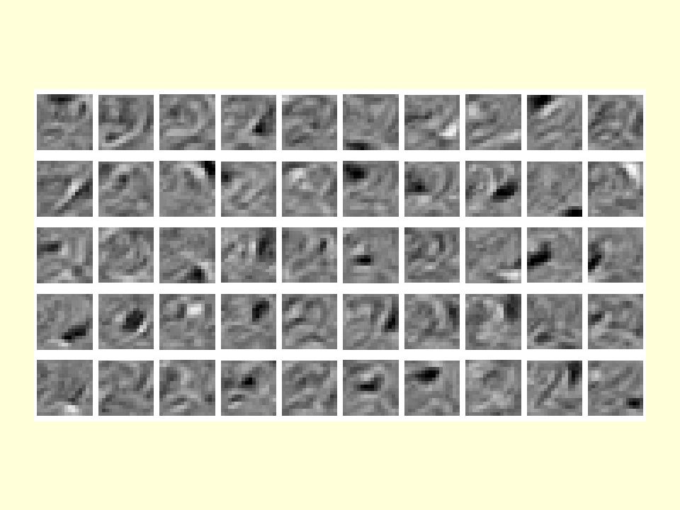
21. The weights of the 50 feature detectors We start with small random weights to break symmetry

38. The final 50 x 256 weights Each neuron grabs a different feature.

39. Reconstruction from activated binary features Data Reconstruction from activated binary features Data How well can we reconstruct the digit images from the binary feature activations? New test images from the digit class that the model was trained on Images from an unfamiliar digit class (the network tries to see every image as a 2) Bush joke 2

40. Training a deep network First train a layer of features that receive input directly from the pixels. Then treat the activations of the trained features as if they were pixels and learn features of features in a second hidden layer. It can be proved that each time we add another layer of features we get a better model of the set of training images. –i.e. we assign lower free energy to the real data and higher free energy to all other possible images. –The proof uses the fact that the variational free energy of a non-equilibrium distribution is always higher that the variational free energy of the equilibrium distribution. –The proof depends on a neat equivalence.

41. Learning the weights in an RBM is exactly equivalent to learning in an infinite causal network with tied weights. A causal network that is equivalent to an RBM v h h 2 v h 1 h 3 etc.

42. First learn with all the weights tied Learning a deep causal network v h1 h 2 v h 1 h 3 etc.

43. Then freeze the bottom layer and relearn all the other layers. h1 h2 v h 1 h 3 etc.

44. Then freeze the bottom two layers and relearn all the other layers. h2 h3 h 2 v h 1 h 3 etc.

45. The generative model after learning 3 layers To generate data: 1.Get an equilibrium sample from the top-level RBM by performing alternating Gibbs sampling. 2.Perform a top-down pass to get states for all the other layers. So the lower level bottom-up connections are not part of the generative model h2 data h1 h3

46. After learning the first layer of weights: If we freeze the generative weights that define the likelihood term and the recognition weights that define the distribution over hidden configurations, we get: Maximizing the RHS is equivalent to maximizing the log prob of “data” that occurs with probability Why the hidden configurations should be treated as data when learning the next layer of weights

47. A neural model of digit recognition 2000 top-level neurons 500 neurons 28 x 28 pixel image 10 label neurons The model learns to generate combinations of labels and images. To perform recognition we do an up- pass from the image followed by a few iterations of the top-level associative memory. The top two layers form an associative memory whose energy landscape models the low dimensional manifolds of the digits. The energy valleys have names

48. Fine-tuning with the up-down algorithm: A contrastive divergence version of wake-sleep Replace the top layer of the causal network by an RBM –This eliminates explaining away at the top-level. –It is nice to have an associative memory at the top. Replace the sleep phase by a top-down pass starting with the state of the RBM produced by the wake phase. –This makes sure the recognition weights are trained in the vicinity of the data. –It also reduces mode averaging. If the recognition weights prefer one mode, they will stick with that mode even if the generative weights like some other mode just as much.

49. SHOW THE MOVIE

50. Examples of correctly recognized handwritten digits that the neural network had never seen before Its very good

51. How well does it discriminate on MNIST test set with no extra information about geometric distortions? Generative model based on RBM’s 1.25% Support Vector Machine (Decoste et. al.) 1.4% Backprop with 1000 hiddens (Platt) 1.6% Backprop with 500 -->300 hiddens 1.6% K-Nearest Neighbor ~ 3.3% Its better than backprop and much more neurally plausible because the neurons only need to send one kind of signal, and the teacher can be another sensory input.

52. Learning perceptual physics Suppose we have a video sequence of some balls bouncing in a box. A physicist would model the data using Newton’s laws. To do this, you need to decide: –How many objects are there? –What are the coordinates of their centers at each time step? –How elastic are they? Does a baby do the same as a physicist? –Maybe we can just learn a model of how the world behaves from the raw video. –It doesn’t learn the abstractions that the physicist has, but it does know what it likes. And what it likes is videos that obey Newtonian physics

53. The conditional RBM model Given the data and the previous hidden state and the previous visible frames, the hidden units at time t are conditionally independent. –So it is easy to sample from their conditional equilibrium distribution. Learning can be done by using contrastive divergence. –Reconstruct the data at time t from the inferred states of the hidden units. –The temporal connections between hiddens can be learned as if they were additional biases t- 2 t- 1 t t- 1 t

54. Show Ilya’s movies

55. THE END For more on this type of learning see: www.cs.toronto.edu/~hinton/science.pdf For the proof that adding extra layers makes the model better see the paper on my web page: “A fast learning algorithm for deep belief nets”

56. Learning with realistic labels This network treats the labels in a special way, but they could easily be replaced by an auditory pathway. 2000 top-level units 500 units 28 x 28 pixel image 10 label units

57. Learning with auditory labels Alex Kaganov replaced the class labels by binarized cepstral spectrograms of many different male speakers saying digits. The auditory pathway then had multiple layers, just like the visual pathway. The auditory and visual inputs shared the top level layer. After learning, he showed it a visually ambiguous digit and then reconstructed the visual input from the representation that the top- level associative memory had settled on after 10 iterations. “six” “five” reconstruction original visual input reconstruction

58. The features learned in the first hidden layer

59. Seeing what it is thinking The top level associative memory has activities over thousands of neurons. –It is hard to tell what the network is thinking by looking at the patterns of activation. To see what it is thinking, convert the top-level representation into an image by using top-down connections. –A mental state is the state of a hypothetical world in which the internal representation is correct. The extra activation of cortex caused by a speech task. What were they thinking? brain state

60. What goes on in its mind if we show it an image composed of random pixels and ask it to fantasize from there? mind brain 2000 top-level neurons 500 neurons 28 x 28 pixel image 10 label neurons

61. data reconstruction feature