Download presentation
Presentation is loading. Please wait.

2
Chapter 5 Statistical Inference Estimation and Testing Hypotheses

3
5.1 Data Sets & Matrix Normal Distribution Data matrix where n rows X 1, …, X n are iid

4
Vec(X') is an np×1 random vector with We writeMore general, we can define matrix normal distribution.
 is an np×1 random vector with We writeMore general, we can define matrix normal distribution.")
5
Definition 5.1.1 An n×p random matrix X is said to follow a matrix normal distributionif where In this case, where W=BB', V=AA', Y has i.i.d. elements each following N(0,1).
..")
6
Theorem 5.5.1 The density function of with W > 0, V >0 is given by where etr(A)= exp(tr(A)). Corollary 1: Let X be a matrix of n observations from Then the density function of X is where

7
5.2 Maximum Likelihood Estimation A. Review Step 1. The likelihood function

8
Step 2. Domain (parameter space) The MLE ofmaximizes over H.
 The MLE ofmaximizes over H.")
9
Step 3. Maximization

10
Results 4.9 (p168 of textbook )
")
11
B. Multivariate population Step 1. The likelihood function Step 2. Domain

12
Step 3. Maximization (a) We can prove that P(B > 0) = 1 if n > p.
 We can prove that P(B > 0) = 1 if n > p.")
13
(b) We have
 We have")
14
(c) Let λ 1, …, λ p be the eigenvalues of Σ *. The function g(λ)= λ -n/2 e -1/ 2λ arrives its maximum at λ=1/n. The function L(Σ * ) arrives its maximum at λ 1 =1/n, …, λ p =1/n and (d) The MLE of Σ is
= λ -n/2 e -1/ 2λ arrives its maximum at λ=1/n. The function L(Σ * ) arrives its maximum at λ 1 =1/n, …, λ p =1/n and (d) The MLE of Σ is.")
15
Theorem 5.2.1 Let X 1, …, X n be a sample from with n > p and. Then the MLEs of are respectively, and the maximum likelihood is

16
Theorem 5.2.2 Under the above notations, we have a) are independent; b) c) is a biased estimator of A unbiased estimator of is recommended by called the sample covariance matrix.
 are independent; b) c) is a biased estimator of A unbiased estimator of is recommended by called the sample covariance matrix.")
17
Matalb code: mean, cov, corrcoef Theorem 5.2.3 Let be the MLE of and be a measurable function. Then is the MLE of. Corollary 1 The MLE of the correlations is

18
5.3 Wishart distribution A. Chi-square distribution Let X 1, …, X n are iid N(0,1). Then, the chi-square distribution with n degrees of freedom or Definition 5.1.1 If x ~ N n (0, I n ), then Y= x ' x is said to have a chi-square distribution with n degrees of freedom, and write.
, then Y= x x is said to have a chi-square distribution with n degrees of freedom, and write..")
19
B. Wishart distribution (obtained by Wishart in 1928) Definition 5.1.1 Let. Then we said that W= x ' x is distributed according to a Wishart distribution.

20
A.Unbiaseness Let be an estimator of. If is called unbiased estimator of. 5.4 Discussion on estimation Theorem 5.4.1 Let X 1, …, X n be a sample from Then are unbiased estimators of and, respectively. Matlab code: mean, cov, corrcoef

21
B. Decision Theory Then the average of loss is give by That is called the risk function.

22
Definition 5.4.2 An estimator t(X) is called a minimax estimator of if Example 1 Under the loss function the sample mean is a minimax estimator of.
 is called a minimax estimator of if Example 1 Under the loss function the sample mean is a minimax estimator of.")
23
C. Admissible estimation Definition 5.4.3 An estimator t 1 (x) is said to be at least as good as another t 2 (x) if And t 1 is said to be better than or strictly dominates t 2 if the above inequality holds with strict inequality for at least one.
 is said to be at least as good as another t 2 (x) if And t 1 is said to be better than or strictly dominates t 2 if the above inequality holds with strict inequality for at least one..")
24
Definition 5.4.4 An estimator t * is said to be inadmissible if there exists another estimator t ** that is better than t *. An estimator t * is admissible if it is not inadmissible. The admissibility is a weak requirement. Under the loss, the sample mean is an inadmissible if the population is James & Stein pointed out is better than The estimator is called James-Stein estimator.

25
5.5 Inferences about a mean vector (Ch.5 Textbook) Let X 1, …, X n be iid samples from Case A: is known. a)p = 1 b)p > 1
p = 1 b)p > 1.")
26
Under the hypothesis H 0, Then Theorem 5.5.1 Let X 1, …, X n be a sample from where is known. The null distribution of under is and the rejection area is

27
Case B: is unknown. a)Suggestion: Replaceby the Sample Covariance Matrix S in, i.e. where Likelihood Ratio Criterion. There are many theoretic approaches to find a suitable statistic. One of the methods is the Likelihood Ratio Criterion.

28
The Likelihood Ratio Criterion (LRC) Step 1The likelihood function Step 2Domains
 Step 1The likelihood function Step 2Domains")
29
Step 3Maximization We have obtained By a similar way we can find where under

30
Then, the LRC is Note

31
Finally Remark: Let t(x) be a statistic for the hypothesis and f(u) is a strictly monotone function. Then is a statistic which is equivalent to t(x). We write
. We write.")
32
5.6 T 2 -statistic Definition 5.6.1 Letandbe independent with n > p. The distribution of is called T 2 distribution. The distribution T 2 is independent of, we shall write As

33
And Theorem 5.6.1 Theorem 5.6.2 The distribution of is invariant under all affine transformations of the observations and the hypothesis

34
Confidence Region A 100 (1- )% confidence region for the mean of a p- dimensional normal distribution is the ellipsoid determined by all such that
% confidence region for the mean of a p- dimensional normal distribution is the ellipsoid determined by all such that")
35
Proof: X 1, …, X n

36
Example 5.6.1 (Example 5.2 in Textbook) Perspiration from 20 healthy females was analysis.
 Perspiration from 20 healthy females was analysis.")
37
Computer calculations provide: and

38
We evaluate Comparing the observedwith the critical value we see thatand consequently, we reject H 0 at the 10% level of significance.

39
Definition 5.6.1 Let x and y be samples of a population G with mean and covariance matrix The quadratic forms are called Mahalanobis distance (M-distance) between x and y, and x and G, respectively. Mahalanobis Distance

40
If can be verified that

41
5.7 Two Samples Problems (Section 6.3, Textbook)
")
42
We have two samples from the two populations where are unknown. The LRC is where

43
Under the hypothesis The confidence region of is where

44
Example 5.7.1(p.338-339) Jolicoeur and Mosimann (1960) studied the relationship of size and shape for painted turtles. The following table contains their measurements on the carapaces of 24 female and 24 male turtles.

46
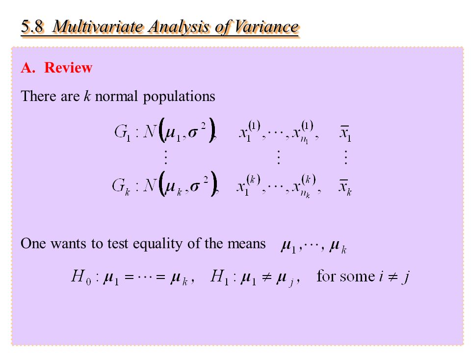
5.8 Multivariate Analysis of Variance A.Review There are k normal populations One wants to test equality of the means

47
The analysis of variance employs decomposition of sum squares where The testing statistics is

48
B.Multivariate population (pp295-305) is unknown, one wants to test
 is unknown, one wants to test")
49
I. The likelihood ratio criterion Step 1The likelihood function Step 2The domains

50
Step 3Maximization where are the total sum of squares and products matrix and the error sum of squares and products matrix, respectively.

51
The treatment sum of squares and product matrix The LRC

52
Definition 5.8.1 Assumeare independent, where. The distribution is called Wilks -distribution and write. Theorem 5.8.1 Under H 0 we have 1) 2) 3) E and B are independent
 2) 3) E and B are independent.")
53
Special cases of the Wilks -distributions See pp300-305, Textbook for example.

54
2.Union-Intersection Decision Rule Consider projection hypothesis

55
For projection data, we have and the F-statistic With the rejection region The rejection region for H 0 is that implies the testing statistic is or

56
Lemma 1Let A be a symmetric matrix of order p. Denote by, the eigenvalues of A, and, the associated eigenvectors of A. Then

57
Lemma 2Let A and B are two p× p matrices and A’ = A, B>0. Denote by and, the eigenvalues of and associated eigenvectors. Then Remark1: Remark2: Remark3: Let be eigenvalues of. The Wilks -statistic can be expressed as

Similar presentations
 2004 Brooks/Cole, a division of Thomson Learning, Inc. Chapter 9 Inferences Based on Two Samples.>")


 Parameter Estimation of PDF and Fitting a Distribution Function.>")


 values must be estimated before.>")


