Download presentation
Presentation is loading. Please wait.

1
Chapter 1: Introduction
Biometrics STAT 319 Chapter 1: Introduction

2
STAT 319 Biometrics Spring 2009
Student Password: A student’s password is their 8-digit tech-id. Standard Form for User-IDs: The standard form for student user-ids is the following: FLastName.Dxxx.yy where F is the first initial of the student, LastName is the last name of the student D is the first letter of the department (M for Math, S for Stat or H for Hons) xxx is the course number yy is the section number Note: all non-alphabetic characters are removed from a student’s First and Last names before forming the user-id. Drive structure: When logged on to a lab or computer classroom computer, drive H: and the My Documents folder, refer to the same folder. This is true for both faculty and students alike. For students, drive I: refers to Class Files folder associated with the class. For faculty, drive I: refers to a folder containing folders for all classes taught by the instructor. In each class folder there is the Class Files folder (that the students see as drive I: ), and a folder for each student in the class where the students can store their work. Instructors can place files that they want students to access in the Class Files folder; students cannot modified or delete files in these folders. STAT Biometrics Spring 2009
 xxx is the course number. yy is the section number. Note: all non-alphabetic characters are removed from a student’s First and Last names before forming the user-id. Drive structure: When logged on to a lab or computer classroom computer, drive H: and the My Documents folder, refer to the same folder. This is true for both faculty and students alike. For students, drive I: refers to Class Files folder associated with the class. For faculty, drive I: refers to a folder containing folders for all classes taught by the instructor. In each class folder there is the Class Files folder (that the students see as drive I: ), and a folder for each student in the class where the students can store their work. Instructors can place files that they want students to access in the Class Files folder; students cannot modified or delete files in these folders. STAT 319 Biometrics Spring")
3
Important Data Sources
Minnesota Department of Health Center for Disease Control (CDC) Australian Bureau of Statistics National Wild Fish Health Survey Bureau of Justice Statistics STAT Biometrics Spring 2009
 Australian Bureau of Statistics. National Wild Fish Health Survey. Bureau of Justice Statistics. STAT 319 Biometrics Spring")
4
STAT 319 Biometrics Spring 2009
1.1 Overview Statistics is a collection of methods for Planning experiments Obtaining data (data are collected observations, such as measurements and survey responses) Organizing data Summarizing (graphically and numerically) data Analyzing data Interpreting results Presenting results, and Drawing conclusions or making inferences Statistics is a branch of Mathematics -> STAT Biometrics Spring 2009
 Organizing data. Summarizing (graphically and numerically) data. Analyzing data. Interpreting results. Presenting results, and. Drawing conclusions or making inferences. Statistics is a branch of Mathematics -> STAT 319 Biometrics Spring")
5
STAT 319 Biometrics Spring 2009
Statistics is invented for studying Randomness- a lack of order, purpose, cause, or predictability (by Wiki)- without which the world will be of no interest. Examples of random phenomena: Phelps won 8 gold medals A 6-sided die is flipped and landed a 4 It’s going to rain tomorrow Randomness, Fuzziness and Uncertainty Randomness creates uncertainty. On the other hand, randomness can be used. When estimating the proportion of current SCSU students who smoked, we can randomly survey 1000 students and use the survey responses as our data. How randomness is used? Why use it? STAT Biometrics Spring 2009
- without which the world will be of no interest. Examples of random phenomena: Phelps won 8 gold medals. A 6-sided die is flipped and landed a 4. It’s going to rain tomorrow. Randomness, Fuzziness and Uncertainty. Randomness creates uncertainty. On the other hand, randomness can be used. When estimating the proportion of current SCSU students who smoked, we can randomly survey 1000 students and use the survey responses as our data. How randomness is used Why use it STAT 319 Biometrics Spring")
6
STAT 319 Biometrics Spring 2009
Population and Sample In the previous example, all SCSU students form a population while the 1000 surveyed form a sample. In general, a population is the complete collection of all items to be studied. These items can be human subjects, animals, machines, even scores. A sample is a sub-collection of items selected from a population. STAT Biometrics Spring 2009

7
STAT 319 Biometrics Spring 2009
More about Samples A sample should represent the underlying population. Therefore, sample data must be collected in an appropriate way, such as through a process of random selection. A self-selected sample is one in which the respondents themselves decide whether to be included. USA Today often publish results from surveys in which people with strong interests or opinions are more likely to participate. The survey responses are not representative of the whole population. Valid conclusions based on a self-selected sample can be made only about the specific group of people who chose to participate. How large should a sample be? What are those appropriate ways to generate a sample? STAT Biometrics Spring 2009

8
Parameter and Statistic
One of the important tasks of statistics is to estimate a quantity for a population. For example, we are interested in the proportion (denoted p) of voters who support presidential candidate X. Here the population consists of all qualified voters and the quantity of interest is p. Another quantity of interest is the average GPA (denoted µ) of all new SCSU students. Here the unknown quantities p and µ are called parameters. STAT Biometrics Spring 2009
 of voters who support presidential candidate X. Here the population consists of all qualified voters and the quantity of interest is p. Another quantity of interest is the average GPA (denoted µ) of all new SCSU students. Here the unknown quantities p and µ are called parameters. STAT 319 Biometrics Spring")
9
Minnesota Teacher Characteristics and Average Salary
97 percent of teachers are licensed 50 percent have advanced degrees 56 percent have taught more than 10 years Average Salary The average salary for a Minnesota public school teacher was $46,906 in 2005; there were 52,213 full-time equivalent teachers. Source: STAT Biometrics Spring 2009

10
STAT 319 Biometrics Spring 2009
The following are all parameters: percent of teachers are licensed percent have advanced degrees percent have taught more than 10 years average salary for a Minnesota public school teacher in 2005 The true values of these parameters are all known by census. STAT Biometrics Spring 2009

11
STAT 319 Biometrics Spring 2009
We now know that a parameter is a quantity associated with a population. To estimate a parameter, one usually takes a sample from the population. A quantity based on the sample, called statistic, can be used to estimate the unknown population quantity. Example: Based on a sample of 877 surveyed executives, it is found that 45% of them would not hire someone with a typographic error on their job application. That figure of 45% is a statistic because it is based on a sample. STAT Biometrics Spring 2009

12
STAT 319 Biometrics Spring 2009
A parameter is a measurement describing some characteristic of a population. A statistic is a measurement describing some characteristic of a sample. STAT Biometrics Spring 2009

13
STAT 319 Biometrics Spring 2009
1.2 Types of Data Data are observations that have been collected. Data can be numerical, such as heights, weights, incomes, GPAs, tumor counts, or Non-numerical, such as colors, genders, smoking status, political affiliations Numerical data are called quantitative data, which consist of numbers representing counts or measurements. Non-numerical data are called qualitative (or categorical) data, which can be separated into different categories. STAT Biometrics Spring 2009
 data, which can be separated into different categories. STAT 319 Biometrics Spring")
14
STAT 319 Biometrics Spring 2009
Types of Data (cont’d) Quantitative data can be discrete or continuous Discrete data are counts, such as the number of bacteria in a bottle of water. Continuous data are measurements that can assume any value over a continuous span, such as the amount of water in a bottle. STAT Biometrics Spring 2009
 Quantitative data can be discrete or continuous. Discrete data are counts, such as the number of bacteria in a bottle of water. Continuous data are measurements that can assume any value over a continuous span, such as the amount of water in a bottle. STAT 319 Biometrics Spring")
15
Four Levels of Measurements
There are 4 levels of measurements Data are at the nominal level of measurement if they can not be arranged in an ordering scheme. Such as colors and genders Data are at the ordinal level of measurement if they are qualitative, but can be arranged in an ordering scheme, such as letter grades STAT Biometrics Spring 2009

16
Four Levels of Measurements (cont’d)
Data are at the interval level of measurement if they are quantitative, but a zero does not mean none, such as temperatures, years Data are at the ratio level of measurement if they are quantitative and a zero does mean none, such as weights, heights, ages, GPAs For interval data, differences are meaningful, while ratios are meaningless. For example, 400F is not twice as hot as 200F. For ratio data, both differences and ratios are meaningful. STAT Biometrics Spring 2009

17
STAT 319 Biometrics Spring 2009
A Data Example This case study is an example of a clinical trial to assess the effectiveness of a new drug as part of a combination therapy (diet, exercise and drug) to treat obesity. Click me to see the data STAT Biometrics Spring 2009
 to treat obesity. Click me to see the data. STAT 319 Biometrics Spring")
18
STAT 319 Biometrics Spring 2009
1.3 Design of Experiments An experiment is a study design in which experimental units are randomly assigned to treatments. Vocabulary Experimental units are individuals on whom an experiment is performed. Usually called subjects or participants when they are human. A treatment is the process, intervention, or other controlled circumstance applied to randomly assigned experimental units. STAT Biometrics Spring 2009

19
STAT 319 Biometrics Spring 2009
Example of Experiment Over a 4-month period, among 30 people with bipolar disorder, patients who were given a high dose (10g/day) of omege-3 fats from fish oil improved more than those given a placebo. Identify the experimental units and treatments used. STAT Biometrics Spring 2009
 of omege-3 fats from fish oil improved more than those given a placebo. Identify the experimental units and treatments used. STAT 319 Biometrics Spring")
20
Observational Studies
An observational study is one in which no manipulation of treatments is employed. In observational studies the researcher doesn’t assign choices but observes outcomes. Widely used in public health and marketing. STAT Biometrics Spring 2009

21
Example of Observational Studies
(Blood pressure) In a test of roughly 200 men and women, those with moderately high blood pressure (averaging 164/89 mm Hg) did worse on tests of memory and reaction time than those with normal blood pressure. (Hypertension 36 [2000]: 1079) STAT Biometrics Spring 2009
 In a test of roughly 200 men and women, those with moderately high blood pressure (averaging 164/89 mm Hg) did worse on tests of memory and reaction time than those with normal blood pressure. (Hypertension 36 [2000]: 1079) STAT 319 Biometrics Spring")
22
Retrospective and Prospective Studies
An observational study can be retrospective or prospective. A retrospective (or case-control) study is one in which subjects are first identified and then their previous conditions or behaviors are determined. A prospective (or cohort) study is one in which subjects are followed to observe future outcomes. STAT Biometrics Spring 2009
 study is one in which subjects are first identified and then their previous conditions or behaviors are determined. A prospective (or cohort) study is one in which subjects are followed to observe future outcomes. STAT 319 Biometrics Spring")
23
STAT 319 Biometrics Spring 2009
Case-Control Studies outcome is measured before exposure controls are selected on the basis of not having the outcome good for rare outcomes relatively inexpensive smaller numbers required quicker to complete prone to selection bias prone to recall/retrospective bias related methods are risk (retrospective), chi-square 2 by 2 test, Fisher's exact test, exact confidence interval for odds ratio, odds ratio meta-analysis and conditional logistic regression. Source: STAT Biometrics Spring 2009
, chi-square 2 by 2 test, Fisher s exact test, exact confidence interval for odds ratio, odds ratio meta-analysis and conditional logistic regression. Source: STAT 319 Biometrics Spring")
24
STAT 319 Biometrics Spring 2009
Cohort Studies outcome is measured after exposure yields true incidence rates and relative risks may uncover unanticipated associations with outcome best for common outcomes expensive requires large numbers takes a long time to complete prone to attrition bias (compensate by using person-time methods) prone to the bias of change in methods over time related methods are risk (prospective), relative risk meta-analysis, risk difference meta-analysis and proportions STAT Biometrics Spring 2009
 prone to the bias of change in methods over time. related methods are risk (prospective), relative risk meta-analysis, risk difference meta-analysis and proportions. STAT 319 Biometrics Spring")
25
Examples of Retrospective and Prospective Studies
A researcher obtains data about head injuries by examining hospital records from the past 5 years. -- retrospective (Psychology of Trauma) A researcher plans to obtain data by following (to the year 2020) siblings of victims who perished in a terrorist attack. -- prospective STAT Biometrics Spring 2009
 A researcher plans to obtain data by following (to the year 2020) siblings of victims who perished in a terrorist attack. -- prospective. STAT 319 Biometrics Spring")
26
STAT 319 Biometrics Spring 2009
More Reading STAT Biometrics Spring 2009

27
Cross-sectional Study
A cross-sectional study involves data collected at a single point in time, often using survey research methods Example: The Centers for Disease Control (CDC) obtains current flu data by polling 3000 people this month. STAT Biometrics Spring 2009
 obtains current flu data by polling 3000 people this month. STAT 319 Biometrics Spring")
28
Differences between Experiments and Observational Studies
Whether treatments are employed Experiments can study causal relationship, but observational studies can NOT. For example, experiments can (but observational studies can NOT) answer questions such as Does taking vitamin C reduce the chance of getting a cold? Is this drug a safe and effective treatment for that disease? STAT Biometrics Spring 2009
 answer questions such as. Does taking vitamin C reduce the chance of getting a cold Is this drug a safe and effective treatment for that disease STAT 319 Biometrics Spring")
29
STAT 319 Biometrics Spring 2009
Study Issues The results of observational studies are considered much less convincing than those of designed experiments, as they are much more prone to selection bias. Researchers attempt to compensate for this with complicated statistical methods such as propensity score matching methods. Experiments may be ruined because of confounding. Confounding occurs when effects of variables are somehow mixed so that the individual effects of the variables can not be identified. STAT Biometrics Spring 2009

30
STAT 319 Biometrics Spring 2009
Example: people are treated with a vaccine designed to prevent Lyme disease caused by ticks.If an early onset of cold weather causes the ticks to hibernate and the 1000 vaccinated subjects subsequently experience an unusually low incidence of Lyme disease, we don’t know if the lower disease rate is the result of an effective vaccine or the early onset of cold weather. The effects of the vaccine and the effects of the cold weather have been mixed and can not be distinguished. A better experimental design would take account of both the vaccine and the cold weather. STAT Biometrics Spring 2009

31
Controlling Effects of Variables
Effects of variables can be controlled by using such devices as Blinding Blocking Randomization STAT Biometrics Spring 2009

32
STAT 319 Biometrics Spring 2009
Blinding In an experimental design to test the effectiveness of a vaccine, some subjects are given such a treatment, while others are given a placebo. A placebo effect occurs when an untreated subject reports an improvement in symptoms. Blinding can minimize a placebo effect. An experiment can be single-blinded or double-blinded. STAT Biometrics Spring 2009

33
STAT 319 Biometrics Spring 2009
Blocking Blocking is the arranging of experimental units in groups (blocks) that are similar to one another. For example, an experiment is designed to test a new drug on patients. In addition to the new drug treatment, a placebo is also administered to male and female patients in a double blind trial. The sex of the patient is a blocking factor accounting for treatment variability between males and females. This reduces sources of variability and thus leads to greater precision. STAT Biometrics Spring 2009
 that are similar to one another. For example, an experiment is designed to test a new drug on patients. In addition to the new drug treatment, a placebo is also administered to male and female patients in a double blind trial. The sex of the patient is a blocking factor accounting for treatment variability between males and females. This reduces sources of variability and thus leads to greater precision. STAT 319 Biometrics Spring")
34
STAT 319 Biometrics Spring 2009
Blocking 30 with treatment 30 with placebo 30 with treatment 30 with placebo Females Males STAT Biometrics Spring 2009

35
STAT 319 Biometrics Spring 2009
Randomization To control effects of variables in an experiment, a third device is to randomly assign subjects to treatments. Randomization tends to balance treatment groups with respect to confounding variables. When assigning subjects, one approach is to use a completely randomized design (CRD), whereby the assignment is done by using a completely random assignment process. For example, Imagine that we have children, a coin, a vaccine, and a placebo. Flip the coin, assign a child to the vaccine if an outcome of heads results, otherwise to the placebo. STAT Biometrics Spring 2009
, whereby the assignment is done by using a completely random assignment process. For example, Imagine that we have children, a coin, a vaccine, and a placebo. Flip the coin, assign a child to the vaccine if an outcome of heads results, otherwise to the placebo. STAT 319 Biometrics Spring")
36
Randomization (cont’d)
CRD is not efficient when blocking factor exists. A more efficient approach is to use a randomized (complete) block design (RCBD). In the previous example, we first form blocks of males and females. Then in each block, we use a CRD. If the vaccine does affect males and females differently, The RCBD has a much better chance to detect that difference. STAT Biometrics Spring 2009
 block design (RCBD). In the previous example, we first form blocks of males and females. Then in each block, we use a CRD. If the vaccine does affect males and females differently, The RCBD has a much better chance to detect that difference. STAT 319 Biometrics Spring")
37
Replication and Sample Size
In addition to controlling effects of variables, another key element of experimental design is the sample size. The larger the sample size in a treatment group, the easier to detect differences from different treatments. Using a same treatment to more than one subjects is called replication. Replication increases the sample size. The subjects using the same treatment are called replicates. STAT Biometrics Spring 2009

38
STAT 319 Biometrics Spring 2009
Sampling Strategies Random sampling: obtaining a sample in such a way that each individual in the population has the same chance of being chosen. A sample thus obtained is called a random sample. A random sample of size n is called a simple random sample (SRS), if any possible sample of the same size n has the same chance of being chosen. STAT Biometrics Spring 2009
, if any possible sample of the same size n has the same chance of being chosen. STAT 319 Biometrics Spring")
39
STAT 319 Biometrics Spring 2009
Example Picture a classroom with 36 students arranged in six rows of 6 students each. Consider two sampling schemes: (1) Write 1 to 36 on 36 slips of paper, different numbers on different slips. Label students 1 to 36. Put the 36 slips in a bag and shuffle. Take out 6 randomly. (2) Roll a fair die and select the row of students corresponding to the outcome. Which scheme results in a SRS? STAT Biometrics Spring 2009
 Write 1 to 36 on 36 slips of paper, different numbers on different slips. Label students 1 to 36. Put the 36 slips in a bag and shuffle. Take out 6 randomly. (2) Roll a fair die and select the row of students corresponding to the outcome. Which scheme results in a SRS STAT 319 Biometrics Spring")
40
Selecting a Simple Random Sample with Random-Digit Table and Software
The question: How can an auditor select 10 accounts to auditor in a school district that has 60 accounts? Using random-digit tables: Number the subjects in the sampling frame by 01, 02, 03, …, 60 (all numbers have 2 digits as 60 does) In a random digit table, such as this, start from any row and any column you like, say row 2 and column 7, select two digits at a time discarding repeated numbers and those that are 00 or larger than 60. This process continues until you get 10 numbers. Columns Rows 1-5 6-10 11-15 16-20 1 30120 13850 81903 56587 2 69696 81799 27328 33287 3 17784 00005 25584 51364 4 35821 49630 87686 53852 5 75763 40570 04655 30679 STAT Biometrics Spring 2009
 In a random digit table, such as this, start from any row and any column you like, say row 2 and column 7, select two digits at a time discarding repeated numbers and those that are 00 or larger than 60. This process continues until you get 10 numbers. Columns. Rows STAT 319 Biometrics Spring")
41
STAT 319 Biometrics Spring 2009
Answer: 17, 99, 27, 32, 83, 32, 87, 17, 78, 40, 00, 05, 25, 58, 45, 13, 64, 35 Tip: record these numbers in order so you know repeats easily STAT Biometrics Spring 2009

42
STAT 319 Biometrics Spring 2009
Systematic Sampling A systematic random sample is one in which sample units are selected at specified intervals. A "random start" is required as a basis for selecting the units for the sample. STAT Biometrics Spring 2009

43
Selecting a Systematic Random Sample
A table of random digits provides an objective method of selecting a "random start." For example, assume that a listing of 50,000 units represents the population from which a systematic random sample of 400 units is desired. The sample size, 400, is 400/50,000 or 1/125 of the population. From the table, select at random a number between 1 and 125 to begin the sample. If the number selected from the table is "64," the sample would consist of every 125th unit on the listing or in the file, beginning with the 64th unit. Thus, if the units in the population are numbered consecutively, the 64th, 189th, 314th, 439th, 564th, etc., units would be drawn as the sample. Such a sample is called a 1 in 125 systematic sample. Questions: (1) Do all the units have the same chance of being selected? If yes, what is the common probability? (2) How to determine the label of the last sample unit? What is it? Adapted from STAT Biometrics Spring 2009
 Do all the units have the same chance of being selected If yes, what is the common probability (2) How to determine the label of the last sample unit What is it Adapted from STAT 319 Biometrics Spring")
44
STAT 319 Biometrics Spring 2009
Example How can we sample 10 houses from a street of 123 houses? Number the houses by 001, 002, …, 123 Since 123/10=12.3, round down to 12, so every 12th house is chosen after a random starting point between 1 and 12 is chosen. If the random starting point is 8, then the houses selected are 8th, 20th, 32th, 44th, 56th, 78th, 90th, 102th and 114th. STAT Biometrics Spring 2009

45
STAT 319 Biometrics Spring 2009
Convenience Sampling Simply collect results that are very easy to get. STAT Biometrics Spring 2009

46
STAT 319 Biometrics Spring 2009
Stratified Sampling Subdivide the population into at least two different subgroups (called strata) that share the same characteristics (such as gender or age bracket), then draw a simple random sample from each stratum. STAT Biometrics Spring 2009
 that share the same characteristics (such as gender or age bracket), then draw a simple random sample from each stratum. STAT 319 Biometrics Spring")
47
STAT 319 Biometrics Spring 2009
Example At a large University a simple random sample of 5 female professors is selected and a simple random sample of 10 male professors is selected. The two samples are combined to give an overall sample of 15 professors. The overall sample is a stratified sample. STAT Biometrics Spring 2009

48
STAT 319 Biometrics Spring 2009
Example Olivia is planning to take a foreign language class. To research how satisfied other students are with their foreign language classes, she decides to take a sample of 20 such students. The university offers classes in four languages: Spanish, German, French, and Japanese. She will select a simple random sample of five students from each language. STAT Biometrics Spring 2009

49
Computing the Mean from a Stratified Sample
Suppose that a population can be stratified into k groups (called strata) containing N1, N2,…, and Nk units, respectively. Suppose a stratified sample is selected, n1 units being from stratum 1, …, and nk units being from stratum k. Denote the means of the k strata by m1, m2, …, and mk, respectively. Then the mean of the stratified sample is defined as Correction has been made. STAT Biometrics Spring 2009
 containing N1, N2,…, and Nk units, respectively. Suppose a stratified sample is selected, n1 units being from stratum 1, …, and nk units being from stratum k. Denote the means of the k strata by m1, m2, …, and mk, respectively. Then the mean of the stratified sample is defined as. Correction has been made. STAT 319 Biometrics Spring")
50
The SURVEYMEANS procedure in SAS
STAT Biometrics Spring 2009

51
Stratified Sampling: Advantages and Disadvantages
- Better coverage of the population - Convenient to administrate - More efficient Disadvantages - Sometimes difficult in identifying appropriate strata STAT Biometrics Spring 2009

52
STAT 319 Biometrics Spring 2009
Cluster Sampling First divide the population area into sections (called clusters), then randomly select some of those clusters, and then choose all the members from those selected clusters. STAT Biometrics Spring 2009
, then randomly select some of those clusters, and then choose all the members from those selected clusters. STAT 319 Biometrics Spring")
53
STAT 319 Biometrics Spring 2009
Example Suppose you are a representative from an athletic organization wishing to find out which sports Grade 11 students are participating in across Canada. It would be too costly and lengthy to survey every Canadian in Grade 11, or even a couple of students from every Grade 11 class in Canada. Instead, 100 schools are randomly selected from all over Canada. STAT Biometrics Spring 2009

54
Cluster Sampling: Advantages and Disadvantages
- Save time - Reduce cost - Does not require an accurate list of the whole population The disadvantages of Cluster Sampling - Less likely to represent the whole population - Do not have total control over the final sample size STAT Biometrics Spring 2009

55
R Codes: Demonstrating SRS Techniques with Animations
sample.srs = function(pop = 1:205, n = 20){ s = floor(sqrt(length(pop))) x = cbind(sort(rep(1:s, s)), rep(1:s, s)) y = length(pop) - s^2 plot(x, xlim = c(1,s), ylim = c(0, s), pch = 20) points(cbind(1:y, 0), pch = 20) for (i in sample(pop, n)){ if (i <= s^2) a = x[i, ] else a = cbind(y[i - s^2], 0) points(a[1], a[2], col = "red", pch = 10, cex = 3) Sys.sleep(0.5) } sample.srs() STAT Biometrics Spring 2009
{ s = floor(sqrt(length(pop))) x = cbind(sort(rep(1:s, s)), rep(1:s, s)) y = length(pop) - s^2. plot(x, xlim = c(1,s), ylim = c(0, s), pch = 20) points(cbind(1:y, 0), pch = 20) for (i in sample(pop, n)){ if (i <= s^2) a = x[i, ] else a = cbind(y[i - s^2], 0) points(a[1], a[2], col = red , pch = 10, cex = 3) Sys.sleep(0.5) } sample.srs() STAT 319 Biometrics Spring")
56
R Codes: Demonstrating Cluster Sampling Techniques with Animations
sample.cluster = function(pop = list(1:20, 1:30, 1:40, 1:50, 1:60), n = 3){ len = sapply(pop, length) k = length(pop) plot(1,1, type = 'n', xlim = c(1, max(len)), ylim = c(1,k)) for (i in 1:k){ for (j in pop[[i]]) points(j, i, pch = 20) } x = sample(1:k, n) for (i in x){ for (j in pop[[i]]){ points(j, i, col = "red", pch = 10, cex = 2); Sys.sleep(0.05) sample.cluster() STAT Biometrics Spring 2009
, n = 3){ len = sapply(pop, length) k = length(pop) plot(1,1, type = n , xlim = c(1, max(len)), ylim = c(1,k)) for (i in 1:k){ for (j in pop[[i]]) points(j, i, pch = 20) } x = sample(1:k, n) for (i in x){ for (j in pop[[i]]){ points(j, i, col = red , pch = 10, cex = 2); Sys.sleep(0.05) sample.cluster() STAT 319 Biometrics Spring")
57
R Codes: Demonstrating Stratified Sampling Techniques with Animations
sample.stratified = function(pop = list(1:20, 1:30, 1:40, 1:50, 1:60), n = 2:6){ len = sapply(pop, length) k = length(pop) plot(1,1, type = 'n', xlim = c(1, max(len)), ylim = c(1,k)) for (i in 1:k){ for (j in pop[[i]]){ points(j, i, pch = 20) } for (i in 1:k) { s = sample(len[i], n[i]) for(j in s) { points(pop[[i]][j], i, col = "red", pch = 10, cex = 2); Sys.sleep(1)} sample.stratified() STAT Biometrics Spring 2009
, n = 2:6){ len = sapply(pop, length) k = length(pop) plot(1,1, type = n , xlim = c(1, max(len)), ylim = c(1,k)) for (i in 1:k){ for (j in pop[[i]]){ points(j, i, pch = 20) } for (i in 1:k) { s = sample(len[i], n[i]) for(j in s) { points(pop[[i]][j], i, col = red , pch = 10, cex = 2); Sys.sleep(1)} sample.stratified() STAT 319 Biometrics Spring")
58
Multistage Sample Designs
A Multistage Sample Design is to combine some of the above five sampling schemes. STAT Biometrics Spring 2009

59
STAT 319 Biometrics Spring 2009
Example In order to select a sample of undergraduate students in the United States, a simple random sample of four states is selected. From each of these states, a simple random sample of two colleges or universities is then selected. Finally, from each of these eight colleges or universities, a simple random sample of 20 undergraduates is selected. The final sample consists of 160 undergraduates. STAT Biometrics Spring 2009

60
STAT 319 Biometrics Spring 2009
Example On a chilly spring afternoon, 10 lab sections of a statistics class all have full attendance. The 10 lab sections each have the same number of students enrolled in it. A class evaluation is about to be administered to some of students. It has been decided to first randomly select 3 of the 10 lab sections and then give the evaluation to a simple random sample of one-fourth of the students in those sections. STAT Biometrics Spring 2009

61
STAT 319 Biometrics Spring 2009
Sampling Errors A sampling error is the difference between a sample result and the true population result. Such an error results from sample-to-sample variation. A non-sampling error occurs when the sample data are incorrectly collected, recorded, and analyzed. STAT Biometrics Spring 2009

62
Chapter 2 Describing, Exploring, and Comparing Data
Biometrics STAT Chapter 2 Describing, Exploring, and Comparing Data

63
STAT 319 Biometrics Spring 2009
2.1 Overview Important Characteristics of Data Center: a representative value that indicates where the middle of the data set is located. Variation: a measure of the amount that the data values vary among themselves. Distribution: The nature or shape of the distribution of the data (such as bell-shaped, uniform, or skewed). Outliers: sample values that lie very far away from the majority of the other sample values. STAT Biometrics Spring 2009
. Outliers: sample values that lie very far away from the majority of the other sample values. STAT 319 Biometrics Spring")
64
Descriptive Statistics and Inferential Statistics
The numerical summaries and graphical summaries to be presented in this chapter are called descriptive statistics. Methods to make inferences about a population using sample data are called inferential statistics. STAT Biometrics Spring 2009

65
2.2 Frequency Distributions
A frequency distribution lists data values (individually for categorical data or by groups or intervals for quantitative data), along with their corresponding frequencies (or counts). Vocabulary: The frequency for a particular category is the number of original values that fall into the category. STAT Biometrics Spring 2009
, along with their corresponding frequencies (or counts). Vocabulary: The frequency for a particular category is the number of original values that fall into the category. STAT 319 Biometrics Spring")
66
STAT 319 Biometrics Spring 2009
Example (categorical data) The array of grades of a statistics class is given below: B B A C B A C C B B A A F D B C A B C B B D The frequency distribution of grades is given in the table. Does the frequency distribution contain the same amount of information as the data does? Grades Frequencies A 5 B 9 C D 2 F 1 STAT Biometrics Spring 2009
 The array of grades of a statistics class is given below: B B A C B A C C B B. A A F D B C A B C B. B D. The frequency distribution of grades is given in the table. Does the frequency distribution contain the same amount of information as the data does Grades. Frequencies. A. 5. B. 9. C. D. 2. F. 1. STAT 319 Biometrics Spring")
67
STAT 319 Biometrics Spring 2009
Example (quantitative data) The systolic blood pressures (SBP) of 20 men are given: The frequency distribution of the data is given in the table. Here: [90,100] means 90 to 100, inclusive, while (100,110] means 100 to 110, excluding 100. Does the frequency distribution contain the same amount of information as the data does? SBP (Interval) Frequency [90,100] 1 (100,110] 4 (110,120] 6 (120,130] (130,140] (140,150] (150,160] Tip: First sort the data from lowest to highest. STAT Biometrics Spring 2009
 The systolic blood pressures (SBP) of 20 men are given: The frequency distribution of the data is given in the table. Here: [90,100] means 90 to 100, inclusive, while (100,110] means 100 to 110, excluding 100. Does the frequency distribution contain the same amount of information as the data does SBP (Interval) Frequency. [90,100] 1. (100,110] 4. (110,120] 6. (120,130] (130,140] (140,150] (150,160] Tip: First sort the data from lowest to highest. STAT 319 Biometrics Spring")
68
Terms Used with Frequency Distributions
Classes are categories (for categorical data) or intervals (for quantitative data). Intervals should have the same length. For quantitative data, we have the following terms: Lower class limits are the smallest numbers that can belong to the different classes. Upper class limits are the largest numbers that can belong to the different classes. Class boundaries are the numbers used to separate classes. Class midpoints are the midpoints of the classes. Class width is the common length of classes. STAT Biometrics Spring 2009
 or intervals (for quantitative data). Intervals should have the same length. For quantitative data, we have the following terms: Lower class limits are the smallest numbers that can belong to the different classes. Upper class limits are the largest numbers that can belong to the different classes. Class boundaries are the numbers used to separate classes. Class midpoints are the midpoints of the classes. Class width is the common length of classes. STAT 319 Biometrics Spring")
69
STAT 319 Biometrics Spring 2009
Example SBP Frequency [90,100] 1 (100,110] 4 (110,120] 6 (120,130] (130,140] (140,150] (150,160] Find -- Classes: Lower Class Limits: Upper Class Limits: Class Midpoints: Class Width: STAT Biometrics Spring 2009

70
STAT 319 Biometrics Spring 2009
Answer SBP Frequency [90,100] 1 (100,110] 4 (110,120] 6 (120,130] (130,140] (140,150] (150,160] Find -- Classes: 7 classes, [90,100],(100,110],… Lower Class Limits:90, 100, 110, …,150 Upper Class Limits: 100, 110, …, 160 Class Midpoints: 95, 105, …, 155 Class Width: 10 STAT Biometrics Spring 2009

71
Procedure for Constructing a Frequency Distribution
Step 1: Decide on the number of classes you want. (5 – 25) Step 2: Calculate the class width (round up) class width (maximum – minimum) / #classes Step 3: Determine the lower class limit of the first class. This number is either the lowest data value or a convenient value that is a little smaller. Step 4: Determine all other lower class limits using the lower class limit of the first class and the class width. Step 5: List all the lower class limits in a vertical column and proceed to enter the upper class limits, which are easily identified. Step 6: Enter the second column of frequencies. STAT Biometrics Spring 2009
 Step 2: Calculate the class width (round up) class width (maximum – minimum) / #classes. Step 3: Determine the lower class limit of the first class. This. number is either the lowest data value or a convenient. value that is a little smaller. Step 4: Determine all other lower class limits using the lower. class limit of the first class and the class width. Step 5: List all the lower class limits in a vertical column and. proceed to enter the upper class limits, which are. easily identified. Step 6: Enter the second column of frequencies. STAT 319 Biometrics Spring")
72
STAT 319 Biometrics Spring 2009
Example Construct the frequency distribution for the 20 systolic blood pressures (SBP) of 20 men using 7 classes. We need to determine- #classes: Class width: The lower limit of the first class: Other lower limits: Upper limits: Frequencies: STAT Biometrics Spring 2009
 of 20 men using 7 classes. We need to determine- #classes: Class width: The lower limit of the first class: Other lower limits: Upper limits: Frequencies: STAT 319 Biometrics Spring")
73
STAT 319 Biometrics Spring 2009
Answer Construct the frequency distribution for the 20 systolic blood pressures (SBP) of 20 men using 7 classes. Solution #classes: 7 Class width: (158 – 93) / 7 = 9.3 10 The lower limit of the first class: 90 Other lower limits: 100, 110, 120, 130, 140, 150 Upper limits: 100, 110, …, 160 Frequencies: See the table SBP Frequency [90,100] 1 (100,110] 4 (110,120] 6 (120,130] (130,140] (140,150] (150,160] STAT Biometrics Spring 2009
 of 20 men using 7 classes. Solution. #classes: 7. Class width: (158 – 93) / 7 = 9.3 10. The lower limit of the first class: 90. Other lower limits: 100, 110, 120, 130, 140, 150. Upper limits: 100, 110, …, 160. Frequencies: See the table. SBP. Frequency. [90,100] 1. (100,110] 4. (110,120] 6. (120,130] (130,140] (140,150] (150,160] STAT 319 Biometrics Spring")
74
Construct Frequency Distributions In Excel
Data Analysis Histogram Specify data ranges and upper class limits (bins) By default, Excel generates frequency distributions. STAT Biometrics Spring 2009
 By default, Excel generates frequency distributions. STAT 319 Biometrics Spring")
75
STAT 319 Biometrics Spring 2009

76
Relative Frequency Distribution
The relative frequency for a class is expressed as percent. relative frequency = (frequency) / (sum of all frequencies) In a frequency distribution, if the frequencies are replaced by relative frequencies, the resultant table is called a relative frequency distribution. STAT Biometrics Spring 2009
 / (sum of all frequencies) In a frequency distribution, if the frequencies are replaced by relative frequencies, the resultant table is called a relative frequency distribution. STAT 319 Biometrics Spring")
77
STAT 319 Biometrics Spring 2009
Examples SBP Frequency Relative Frequency [90,100] 1 1/20 = 5% (100,110] 4 4 / 20 = 20% (110,120] 6 6 / 20 = 30% (120,130] 4 /20 = 20% (130,140] (140,150] 0 / 20 = 0% (150,160] 1 /20 = 5% Grades Frequency Relative Frequency A 5 5/22 = B 9 9/22 = C 5/22 D 2 2/22 F 1 1/22 STAT Biometrics Spring 2009

78
Cumulative Frequency Distribution for a Quantitative Variable
The cumulative frequency for a class is the sum of the frequencies for that class and all previous classes. A cumulative frequency distribution lists the intervals that are expressed as “less than or equal to x”, along with the number of values falling in the corresponding intervals. Those x’s are chosen to be the upper class limits. STAT Biometrics Spring 2009

79
STAT 319 Biometrics Spring 2009
Example SBP Cumulative Frequency ≤ 100 1 ≤ 110 5 ≤ 120 11 ≤ 130 15 ≤ 140 19 ≤ 150 ≤ 160 20 (the total) STAT Biometrics Spring 2009
 STAT 319 Biometrics Spring")
80
STAT 319 Biometrics Spring 2009
Example Construct the cumulative frequency distribution that corresponds to the given frequency distribution. Cholesterol of Men Frequency [0,200] 1 (200,400] 5 ( ] 11 ( ] 15 ( ] 19 ( ] ( ] 20 Cholesterol of Men Cumulative Frequency ≤ 200 1 ≤ 400 6 ≤ 600 17 ≤ 800 32 ≤ 1000 51 ≤ 1200 70 ≤ 1400 90 (total) STAT Biometrics Spring 2009
 STAT 319 Biometrics Spring")
81
Cumulative Relative Frequency Distribution for a Quantitative Variable
Cholesterol of Men Cumulative Frequency Cumulative Relative Frequency ≤ 200 1 1/90 = 1.11% ≤ 400 6 6/90 = ≤ 600 17 17/90 = ≤ 800 32 32/90 = ≤ 1000 51 51/90 = ≤ 1200 70 70/90 = ≤ 1400 90 (total) 90/90 = 100% STAT Biometrics Spring 2009
 90/90 = 100% STAT 319 Biometrics Spring")
82
STAT 319 Biometrics Spring 2009
2.3 Visualizing Data Graphs to be constructed: Histogram Ogive Dotplot Stem-and-leaf plot Pareto chart Pie chart Scatterplot Time-series graph STAT Biometrics Spring 2009

83
STAT 319 Biometrics Spring 2009
Histograms A histogram is a bar graph in which the horizontal scale represents classes/intervals of data values and the vertical scale represents frequencies (or relative frequencies). The heights of the bars correspond to the frequency (or the relative frequency) values, and the bars are drawn adjacent to each other without gaps. STAT Biometrics Spring 2009
. The heights of the bars correspond to the frequency (or the relative frequency) values, and the bars are drawn adjacent to each other without gaps. STAT 319 Biometrics Spring")
84
STAT 319 Biometrics Spring 2009
Example Construct a histogram for the 20 systolic blood pressures (SBP) of 20 men SBP Frequency [90,100] 1 (100,110] 4 (110,120] 6 (120,130] (130,140] (140,150] (150,160] STAT Biometrics Spring 2009
 of 20 men SBP. Frequency. [90,100] 1. (100,110] 4. (110,120] 6. (120,130] (130,140] (140,150] (150,160] STAT 319 Biometrics Spring")
85
STAT 319 Biometrics Spring 2009
R Codes SBP = c(93,104,105,108,109,112,114,115,117,119, 119,120,121,123,127,130,135,139,139,158) hist(SBP, breaks = seq(90, 160, 10), col = 'green‘) Copy and paste these codes to R, then you will see the histogram. STAT Biometrics Spring 2009
 hist(SBP, breaks = seq(90, 160, 10), col = green‘) Copy and paste these codes to R, then you will see the histogram. STAT 319 Biometrics Spring")
86
STAT 319 Biometrics Spring 2009
Frequency Polygons A frequency polygon uses line segments connected to points located directly above class midpoint values. The line segments are extended to the right and left so that the graph begins and ends on the horizontal axis. STAT Biometrics Spring 2009

87
STAT 319 Biometrics Spring 2009
SBP Frequency 1 [90,100] 4 (100,110] 6 (110,120] (120,130] (130,140] (140,150] Class midpoints: 94.5, 104.5, 114.5, 124.5, 134.5, 144.5, 154.5 STAT Biometrics Spring 2009

88
STAT 319 Biometrics Spring 2009

89
STAT 319 Biometrics Spring 2009
Dot plots: Shows a dot for each observation, placed just above the value on the number line for that observation. Example Dot plot Quiz scores for twenty students: 5, 7, 8, 3, 7, 7, 1, 9, 6, 8, 5, 6, 7, 10, 7, 9, 6, 8, 6, 6 STAT Biometrics Spring 2009

90
STAT 319 Biometrics Spring 2009
Stem-and-Leaf Plots Stem-and-Leaf Plots: similar to dot plot. Each observation is represented by a stem and a leaf. STAT Biometrics Spring 2009

91
STAT 319 Biometrics Spring 2009
Example Stem-and-Leaf Plot Test scores for 12 students: 80, 45, 100, 76, 84, 87, 96, 62, 75,74, 87, 76 Step 1: Sorted test scores: 45, 62, 74, 75, 76, 76, 80, 84, 87, 87, 96, 100 Step 2: Place the scores in the corresponding stems and leaves. (usually the last digit will be the leaf) Stem Leaves 4 5 6 7 8 9 10 5 2 6 STAT Biometrics Spring 2009
 Stem Leaves STAT 319 Biometrics Spring")
92
STAT 319 Biometrics Spring 2009
Example Quiz scores for 12 students: 8.0, 4.5, 10.0, 7.6, 8.4, 8.7, 9.6, 6.2, 7.5, 7.4, 8.7, 7.6 Step 1: Sorted test scores: 4.5, 6.2, 7.4, 7.5, 7.6, 7.6, 8.0, 8.4, 8.7, 8.7, 9.6, 10.0 Step 2: Place the scores in the corresponding stems and leaves. (usually the last digit will be the leaf) Stem Leaves 4. 5. 6. 7. 8. 9. 10. 5 2 6 STAT Biometrics Spring 2009
 Stem Leaves STAT 319 Biometrics Spring")
93
STAT 319 Biometrics Spring 2009
Pareto Chart: Bar Graph with categories Ordered by Their Frequency from the Tallest Bar to Shortest. Click to see data. STAT Biometrics Spring 2009

94
STAT 319 Biometrics Spring 2009
Pie Charts Pie chart: A circle having a “slice of a pie” for each category. The size of slice corresponds to the percentage of observations in the category. STAT Biometrics Spring 2009

95
STAT 319 Biometrics Spring 2009
Constructing Pareto Chart Using Excel Click to see data STAT Biometrics Spring 2009

96
STAT 319 Biometrics Spring 2009
Scatterplots Is a plot of paired (x,y) data with a horizontal x-axis and a vertical y-axis. Click to see an example. STAT Biometrics Spring 2009
 data with a horizontal x-axis and a vertical y-axis. Click to see an example. STAT 319 Biometrics Spring")
97
STAT 319 Biometrics Spring 2009

98
STAT 319 Biometrics Spring 2009
Time Series A time series is a data set collected over time. STAT Biometrics Spring 2009

99
STAT 319 Biometrics Spring 2009
2.4 Measures of Center A measure of center is a value at the center or middle of a data set. Measures of center: Mean: the average value of data points. Median: the middle value when a data set is arranged in order of magnitude. STAT Biometrics Spring 2009

100
STAT 319 Biometrics Spring 2009
Examples: Find the mean and median of the data: 12, 10, 4, 5, 1 (2) Find the mean and median of the data: 12, 10, 4, 5, 1, 1000 STAT Biometrics Spring 2009
 Find the mean and median of the data: 12, 10, 4, 5, 1, STAT 319 Biometrics Spring")
101
STAT 319 Biometrics Spring 2009
Mode The mode of a data set is the value that occurs most frequently. Examples: The data 2, 2, 3, 1, 5 have a mode of 2 The data 3, 1, 3, 1, 5, 0, 6 have two modes 1 and 3 The data 2, 4, 6, 7, 0 have no mode (no value repeated). STAT Biometrics Spring 2009
. STAT 319 Biometrics Spring")
102
STAT 319 Biometrics Spring 2009
Rounding-off Rule To get more accurate results, carry as many decimal places as possible. STAT Biometrics Spring 2009

103
STAT 319 Biometrics Spring 2009
Weighted Means To calculate a final score, exam 1 accounts for 25%, exam 2 accounts for 35%, and final exam accounts for 40%. Suppose exam 1 is worth 60 points, exam 2 is 80 points, and final exam is 90 points, the final score is the weighted mean (60)(.25) + (80)(.35) + (90)(.40) = 79 STAT Biometrics Spring 2009
(.25) + (80)(.35) + (90)(.40) = 79. STAT 319 Biometrics Spring")
104
STAT 319 Biometrics Spring 2009
Mean or Median Means are sensitive to outliers, while medians are resistant. Means are generally good, but use medians when there is any outlier. STAT Biometrics Spring 2009

105
STAT 319 Biometrics Spring 2009
Mean, Median, and Mode These pictures are smoothed histograms. The distribution of data is Symmetric The distribution is skew to the left The distribution is skew to the right STAT Biometrics Spring 2009

106
STAT 319 Biometrics Spring 2009
2.5 Measures of Variation Range of data: maximum - minimum Standard deviation: measure of variation about the mean Variance: Square of standard deviation All these measure how concentrate (or divergent) the data are. STAT Biometrics Spring 2009
 the data are. STAT 319 Biometrics Spring")
107
STAT 319 Biometrics Spring 2009
Calculation of Variances The variance of a set of observations is an average of the squares of deviation from the mean. The standard deviation s is the square root of the variance STAT Biometrics Spring 2009

108
STAT 319 Biometrics Spring 2009
The standard deviation: Example Example (Calculating the standard deviation s) Metabolic rates of 7 men who took part in a study of dieting. The units are calories per 24 hours. Find the mean first: STAT Biometrics Spring 2009
 Metabolic rates of 7 men who took part in a study of dieting. The units are calories per 24 hours Find the mean first: STAT 319 Biometrics Spring")
109
STAT 319 Biometrics Spring 2009
Cont’d Observations Deviations Squared deviations 1792 192 36864 1666 66 4356 1362 -238 56644 1614 14 196 1460 -140 19600 1867 267 71289 1439 -161 25921 sum = sum = The variance The standard deviation STAT Biometrics Spring 2009

110
Variance and Standard Deviation of a Population
STAT Biometrics Spring 2009

111
Coefficient of Variation (CV)
For a population, For a sample, STAT Biometrics Spring 2009

112
STAT 319 Biometrics Spring 2009
Example: Find CV for the data: 2, 4, 1, 6, 7, 0, 3, 2. mean = ( )/8 = 3.125 Standard deviation = 2.416 CV = 2.416/3.125 = = 77.3% STAT Biometrics Spring 2009
/8 = Standard deviation = CV = 2.416/3.125 = = 77.3% STAT 319 Biometrics Spring")
113
Using Standard Deviation As a Ruler
If a value is within 2 standard deviations away from the mean, then the value is said to be usual. Then, (called the range rule of thumb) The minimum usual value would be mean – 2(standard deviation) The maximum usual value would be mean + 2(standard deviation) STAT Biometrics Spring 2009
 The minimum usual value would be. mean – 2(standard deviation) The maximum usual value would be. mean + 2(standard deviation) STAT 319 Biometrics Spring")
114
STAT 319 Biometrics Spring 2009
Example (Head Circumferences of Girls) Past results from the National Health Survey suggest that the head of circumferences of two-month-old girl have a mean of cm and a standard deviation of 1.64 cm. (1) Use the range rule of thumb to find the minimum and maximum “usual” head circumferences. (2) Determine whether a circumference of 42.6 cm would be considered “unusual”. STAT Biometrics Spring 2009
 Past results from the National Health Survey suggest that the head of circumferences of two-month-old girl have a mean of cm and a standard deviation of 1.64 cm. (1) Use the range rule of thumb to find the minimum and maximum usual head circumferences. (2) Determine whether a circumference of 42.6 cm would be considered unusual . STAT 319 Biometrics Spring")
115
STAT 319 Biometrics Spring 2009
Chebyshev's theorem At least 100(1-1/k^2)% of all values are within k standard deviations of the mean. This is true for any data. STAT Biometrics Spring 2009
% of all values are within k standard deviations of the mean. This is true for any data. STAT 319 Biometrics Spring")
116
68-95-99.7 Rule for Data with a Bell-Shaped Distribution
This rule is also called the empirical rule. This rule states that, for data sets having a distribution that is approximately bell-shaped, About 68% of all values fall within 1 standard deviation of the mean. About 95% of all values fall within 2 standard deviation of the mean. About 99.7% of all values fall within 3 standard deviation of the mean. STAT Biometrics Spring 2009

117
STAT 319 Biometrics Spring 2009
Example (Heights of Women) Heights of women have a bell-shaped distribution with mean 163 cm and standard deviation 6 cm. Then (1) 68% of women have heights between 163 – 1(6) = 157 cm and (6) = 169 cm. (2) 95% of women have heights between 163 – 2(6) = 151 cm and (6) = 175 cm. (3) 99.7% of women have heights between 163 – 3(6) = 145 cm and (6) = 181 cm. STAT Biometrics Spring 2009
 Heights of women have a bell-shaped distribution with mean 163 cm and standard deviation 6 cm. Then. (1) 68% of women have heights between. 163 – 1(6) = 157 cm and (6) = 169 cm. (2) 95% of women have heights between. 163 – 2(6) = 151 cm and (6) = 175 cm. (3) 99.7% of women have heights between. 163 – 3(6) = 145 cm and (6) = 181 cm. STAT 319 Biometrics Spring")
118
2.6 Measures of Relative Standing
A standard score, or z-score, is the number of standard deviation that a given value x is above or below the mean. For a given value x, its z-score is STAT Biometrics Spring 2009

119
Z-scores Can be Used to Compare Values
Example (Heights of Women) Heights of women have a bell-shaped distribution with mean 163 cm and standard deviation 6 cm. Then (1) A woman of 149cm has a z-score of (149 – 163)/6 = (2) A woman of 169cm has a z-score of (169 – 163)/6 = 1 (3) A woman of 178 cm has a z-score of (178 – 163)/6 = 2.5 STAT Biometrics Spring 2009
 Heights of women have a bell-shaped distribution with mean 163 cm and standard deviation 6 cm. Then. (1) A woman of 149cm has a z-score of. (149 – 163)/6 = (2) A woman of 169cm has a z-score of. (169 – 163)/6 = 1. (3) A woman of 178 cm has a z-score of. (178 – 163)/6 = 2.5. STAT 319 Biometrics Spring")
120
Z-Scores and Unusual Values
Usual values have z-scores between – 2 and 2, inclusive. Unusual values have z-scores greater than 2 or less than – 2. If a value has a negative z-score, the value must be less than the mean. Similarly, If a value has a positive z-score, the value must be greater than the mean. STAT Biometrics Spring 2009

121
STAT 319 Biometrics Spring 2009
Example (Heights of Women) Heights of women have a bell-shaped distribution with mean 163 cm and standard deviation 6 cm. The height of a woman is 179cm. Is she unusually tall? Solution: The z-score of 179 cm is (179 – 163)/6 = 2.67, so, she is unusually tall relative to other women. STAT Biometrics Spring 2009
 Heights of women have a bell-shaped distribution with mean 163 cm and standard deviation 6 cm. The height of a woman is 179cm. Is she unusually tall Solution: The z-score of 179 cm is. (179 – 163)/6 = 2.67, so, she is unusually tall relative to other women. STAT 319 Biometrics Spring")
122
STAT 319 Biometrics Spring 2009
Example (Comparing Test Scores) Which is relatively better: A score of 85 on a biology test or a score of 45 on an economics test? Scores on the biology test have a mean of 90 and a standard deviation of 10. Score on the economics test have a mean of 55 and a standard deviation of 5. STAT Biometrics Spring 2009
 Which is relatively better: A score of 85 on a biology test or a score of 45 on an economics test Scores on the biology test have a mean of 90 and a standard deviation of 10. Score on the economics test have a mean of 55 and a standard deviation of 5. STAT 319 Biometrics Spring")
123
STAT 319 Biometrics Spring 2009
Example (Conversion Between Scores) Many colleges and universities accept SAT or ACT scores for admission. Suppose that to have a SAT score in the top 25%, one needs to score at least If one took the alternative ACT test, how high would he need to score in order to make him equivalent to those top 25% SAT scorers. For SAT scores, the mean is 1520 and the standard deviation is 250.For ACT, the mean is 20.8 and the standard deviation is 4.8. STAT Biometrics Spring 2009
 Many colleges and universities accept SAT or ACT scores for admission. Suppose that to have a SAT score in the top 25%, one needs to score at least If one took the alternative ACT test, how high would he need to score in order to make him equivalent to those top 25% SAT scorers. For SAT scores, the mean is 1520 and the standard deviation is 250.For ACT, the mean is 20.8 and the standard deviation is 4.8. STAT 319 Biometrics Spring")
124
Quantiles: Quartiles and Percentiles
Example (SAT Scores) A SAT has three 800-point sections (math, critical reading, and writing). In addition to their score, students receive a number which is the percent of other test takers with lower scores. We are interested in two questions What is the lowest score one should get to be among the top p percent? Say p = 5. If a student’s score is x, what percent of test takers score less than or equal to x? STAT Biometrics Spring 2009
 A SAT has three 800-point sections (math, critical reading, and writing). In addition to their score, students receive a number which is the percent of other test takers with lower scores. We are interested in two questions. What is the lowest score one should get to be among the top p percent Say p = 5. If a student’s score is x, what percent of test takers score less than or equal to x STAT 319 Biometrics Spring")
125
STAT 319 Biometrics Spring 2009
Percentiles The first question is related to percentiles. A percentile is the value below which a certain percent of observations fall. For example, the 20th percentile is the value (or score) below which 20 percent of the observations may be found. In general, the kth percentile of a sample or population is the value (or score) below which k percent of the observations may be found. STAT Biometrics Spring 2009
 below which 20 percent of the observations may be found. In general, the kth percentile of a sample or population is the value (or score) below which k percent of the observations may be found. STAT 319 Biometrics Spring")
126
STAT 319 Biometrics Spring 2009
Quartiles If k = 25, the percentile is called the first quartile, denoted Q1. If k = 50, the percentile is called the second quartile, denoted Q2. If k = 75, the percentile is called the third quartile, denoted Q3. Note that Q2 is just the median. The middle 50% of values are between Q1 and Q3. Inter quartile range: IQR = Q3 - Q1. Percentiles and quartiles are examples of quantiles. STAT Biometrics Spring 2009

127
Finding kth Percentile
Let n = # of data values L = locator that gives the position of a value For example, the 13th value in the sorted data (from smallest to largest) has L = 13. Pk = kth percentile Then L = (k/100)*n. If L is a whole number, Pk = the average of the Lth value and the (L+1)th in the sorted data; Otherwise, round L up to the next whole number, say M, and Pk = Mth value in the sorted data. STAT Biometrics Spring 2009
 has L = 13. Pk = kth percentile. Then. L = (k/100)*n. If L is a whole number, Pk = the average of the Lth value and the (L+1)th in the sorted data; Otherwise, round L up to the next whole number, say M, and Pk = Mth value in the sorted data. STAT 319 Biometrics Spring")
128
STAT 319 Biometrics Spring 2009
Example (Cotinine Levels of 40 Smokers) 0, 1, 1, 3, 17, 32, 35, 44, 48, 86, 87, 103, 112, 121, 123, 130, 131, 149, 164, 167, 173, 173, 198, 208, 210, 222, 227, 234, 245, 250, 253, 265, 266, 277, 284, 289, 290, 313, 477, 491 Find P20 , P25, P75, and IQR. Solution: To find P20, we know n = 40, k = 20. Then L = (k/100)*n = (20/100)*40 = 8. The 20th percentile P20 is then the average of 44 (the 8th) and 48 (the 9th), or 46. STAT Biometrics Spring 2009
 0, 1, 1, 3, 17, 32, 35, 44, 48, 86, 87, 103, 112, 121, 123, 130, 131, 149, 164, 167, 173, 173, 198, 208, 210, 222, 227, 234, 245, 250, 253, 265, 266, 277, 284, 289, 290, 313, 477, 491. Find P20 , P25, P75, and IQR. Solution: To find P20, we know n = 40, k = 20. Then L = (k/100)*n = (20/100)*40 = 8. The 20th percentile P20 is then the average of 44 (the 8th) and 48 (the 9th), or 46. STAT 319 Biometrics Spring")
129
Different Software Packages May Give Different Quantiles
To find the 25th percentile of the data 1, 3, 6, 10, 15, 21, 28, 36 Using the formula, we get 4.5. SAS gives 4.5, too. Excel uses percentile(array, k), click me. The 25th percentile is 5.25. R gives the same result 5.25, x=c(1, 3, 6, 10, 15, 21, 28, 36); quantile(x,0.25) The secret: Both Excel and R use linear interpolation, while SAS takes average. STAT Biometrics Spring 2009
, click me. The 25th percentile is R gives the same result 5.25, x=c(1, 3, 6, 10, 15, 21, 28, 36); quantile(x,0.25) The secret: Both Excel and R use linear interpolation, while SAS takes average. STAT 319 Biometrics Spring")
130
2.7 Exploratory Data Analysis (EDA)
EDA is the process of using statistical tools, numerical or graphical, to investigate data sets in order to understand their important characteristics, such as the center, variation, distribution, and outliers. STAT Biometrics Spring 2009

131
The 5-Number Summary and Boxplots
For a data set, the 5-number summary consists of the minimum value, Q1, Q2, Q3, and the maximum value. A (regular) boxplot is a graphical display of the 5-number summary. STAT Biometrics Spring 2009
 boxplot is a graphical display of the 5-number summary. STAT 319 Biometrics Spring")
132
Procedure for Constructing a Regular Boxplot
Find the 5-number summary. Construct a scale with values that include the minimum and maximum data values. Construct a box extending from Q1 to Q3, and draw a line in the box at the median. Draw lines extending outward from the box to the minimum and maximum data values. STAT Biometrics Spring 2009

133
Procedure for Constructing a Modified Boxplot
Find the 5-number summary. Construct a scale with values that include the minimum and maximum data values. Construct a box extending from Q1 to Q3, and draw a line in the box at the median. Draw lines extending outward from the box to the minimum and maximum data values within the fences formed by Q1 – 1.5*IQR and Q *IQR. (5) Any data values outside the fences are treated as potential outliers and marked in the boxplot. Note: Most software gives modified boxplots. STAT Biometrics Spring 2009
 Any data values outside the fences are treated as potential outliers and marked in the boxplot. Note: Most software gives modified boxplots. STAT 319 Biometrics Spring")
134
STAT 319 Biometrics Spring 2009
Interpretation: The following observations can be made. Means: Variation: Distributions: Outliers: STAT Biometrics Spring 2009

135
Biometrics STAT Chapter 3 Probability

136
False Positives and False Negatives
Example: In clinical trials of a blood test for pregnancy, 99 women are randomly selected from a population of women who seek medical help in determining whether they are pregnant. STAT Biometrics Spring 2009

137
Pregnancy Test Results
Positive Negative Subject is pregnant Subject is not pregnant 5 80 subjects are true positives; 11 subjects are true negatives; 3 subjects are false positives; 5 subjects are false negatives. STAT Biometrics Spring 2009

138
STAT 319 Biometrics Spring 2009
3-1 Overview Rare Event Rule for inferential statistics: If , under a given assumption, the probability of a particular observed event is extremely small, we conclude that the assumption is probably not correct. STAT Biometrics Spring 2009

139
STAT 319 Biometrics Spring 2009
3-2 Fundamentals An event is any collection of results or outcomes of a procedure. A simple event is an event that can not be further broken down into simpler components. The sample space for a procedure consists of all possible simple events. STAT Biometrics Spring 2009

140
STAT 319 Biometrics Spring 2009
Examples of events and sample spaces In the procedure of rolling a die, possible simple events are “rolling a 1”, “rolling a 2”,..., “rolling a 6”. The sample space (S) is the collection of 1, 2, ..., 6, or S = {1,2,...,6}. Is “rolling an even number” a simple event? In the procedure of selecting a ball from a bag which contains 5 balls, 2 red and 3 blue. Possible simple events are “selecting a red ball” and “selecting a blue ball”. The sample space (S) is S = {red, blue}. STAT Biometrics Spring 2009
 is the collection of 1, 2, ..., 6, or S = {1,2,...,6}. Is rolling an even number a simple event In the procedure of selecting a ball from a bag which contains 5 balls, 2 red and 3 blue. Possible simple events are selecting a red ball and selecting a blue ball . The sample space (S) is S = {red, blue}. STAT 319 Biometrics Spring")
141
STAT 319 Biometrics Spring 2009
Notation Events are denoted by upper case letters, such as A, B, C, and so on. P(A) denotes the probability that the event A happens. STAT Biometrics Spring 2009
 denotes the probability that the event A happens. STAT 319 Biometrics Spring")
142
Three Approaches of Defining a Probability
Relative frequency approach: If the event A occurs k times among n trials, then the probability that A occurs, P(A), can be estimated as follows: P(A) = k/n. This approach is based on the Law of Large Numbers. Classical approach: Assume that a given procedure has n different simple events, each of which has an equal chance of occurring. If event A can occur in s of these n ways, then P(A) = s/n. Subjective probability: The probability of an event A, P(A), is estimated by educated guess. STAT Biometrics Spring 2009
, can be estimated as follows: P(A) = k/n. This approach is based on the Law of Large Numbers. Classical approach: Assume that a given procedure has n different simple. events, each of which has an equal chance of occurring. If. event A can occur in s of these n ways, then P(A) = s/n. Subjective probability: The probability of an event A, P(A), is estimated by. educated guess. STAT 319 Biometrics Spring")
143
Law of Large Numbers (LLN)
The relative frequency approach is based on the following theorem: Law of Large Numbers As a procedure is repeated again and again, the relative frequency probability of an event tends to approach the actual probability. STAT Biometrics Spring 2009

144
STAT 319 Biometrics Spring 2009
Simulating LLN LLN can be simulated using Excel. Click to see details. Using R: Copy the following R codes and paste to R GUI x = sample(1:6, 1000, replace = TRUE) freq1 = sum(x==1)/1000 freq1 STAT Biometrics Spring 2009
 freq1 = sum(x==1)/1000. freq1. STAT 319 Biometrics Spring")
145
STAT 319 Biometrics Spring 2009
Examples of Probabilities: Indicating What Approach You are using to Find Probabilities A fair coin is rolled 1000 times, 489 being heads. Estimate the probability of rolling heads. Randomly select a card from a deck of 52 cards. What is the probability of selecting (1) a diamond (2) a face card (3) an ace (4) a card that is not club. What is the probability that it will be raining tomorrow? STAT Biometrics Spring 2009
 a diamond (2) a face card (3) an ace (4) a card that is not club. What is the probability that it will be raining tomorrow STAT 319 Biometrics Spring")
146
Summary: Finding Probabilities Using the Classical Approach
Step 1: Write the sample space to find the number of simple events, n. Step 2: Express the event for which you wish to find a probability in terms of simple events. Find the number of simple events in this event, k. Step 3: The probability is k/n. STAT Biometrics Spring 2009

147
More Examples of Finding Probabilities
A couple plans to have 3 children. Find the probability of each event. (1) Among 3 children, there is exactly one girl. (2) Among 3 children, there are exactly two girls. (3) Among 3 children, all are girls. STAT Biometrics Spring 2009
 Among 3 children, there is exactly one girl. (2) Among 3 children, there are exactly two girls. (3) Among 3 children, all are girls. STAT 319 Biometrics Spring")
148
Basic Properties of Probability
The probability of an impossible event is 0. The probability of an event that is certain to occur is 1. For any event A, 0 ≤ P(A) ≤ 1. STAT Biometrics Spring 2009
 ≤ 1. STAT 319 Biometrics Spring")
149
STAT 319 Biometrics Spring 2009
Complementary Events STAT Biometrics Spring 2009

150
STAT 319 Biometrics Spring 2009
Example Randomly select a card from a deck of 52 cards. What is the probability of selecting a card that is not an ace. STAT Biometrics Spring 2009

151
STAT 319 Biometrics Spring 2009
3-3 Addition Rule A compound event is an event that combines two or more simple events. When tossing a die, the event “tossing an even number” is an example of compound event. When finding the probability of a compound event, we need the addition rule, stated below. Addition Rule Suppose that a compound event A can be expressed as B or C, that is, A = B or C, then P(A) = P(B or C) = P(B) + P(C) - P(B and C). STAT Biometrics Spring 2009
 = P(B or C) = P(B) + P(C) - P(B and C). STAT 319 Biometrics Spring")
152
STAT 319 Biometrics Spring 2009
P(B or C) = P(B) + P(C) - P(B and C) Can be written as P(B C) = P(B) + P(C) - P(B C) STAT Biometrics Spring 2009
 = P(B) + P(C) - P(B and C) Can be written as. P(B C) = P(B) + P(C) - P(B C) STAT 319 Biometrics Spring")
153
STAT 319 Biometrics Spring 2009
Example The following table summarizes blood groups and Rh types for 100 typical people. Blood Group O A B AB Positive Negative Rh Type If one person is randomly selected, find the probability of getting someone who is type Rh -. If one person is randomly selected, find the probability of getting someone who is group B. If one person is randomly selected, find the probability of getting someone who is group B or type Rh -. STAT Biometrics Spring 2009

154
Special Case of the Addition Rule
If two events B and C are disjoint (or mutually exclusive), meaning that they can not occur simultaneously, then P(BC) = P(B) + P(C). STAT Biometrics Spring 2009
, meaning that they can not occur simultaneously, then. P(BC) = P(B) + P(C). STAT 319 Biometrics Spring")
155
Examples of Disjoint Events
Toss a die. Let A = “tossing a 1” and B = “tossing an even number”. A and B are disjoint events. Select a card from a deck of 52. Let A = “a Jack”, B = “a 4”, and C = “Not a club”. A and B are disjoint, but neither A nor B is disjoint with C. Find (1) P(A or B) (2) P(A or C) (3) P(B or C) STAT Biometrics Spring 2009
 P(A or B) (2) P(A or C) (3) P(B or C) STAT 319 Biometrics Spring")
156
3-4 Multiplication Rule: Basics
Notation P(A and B) = P(event A and event B occurs simultaneously) P(A and B) can be written as P(AB). P( B | A ) = P(event B occurs, given that event A has already ocurred.) P(AB) = P(A)P(B|A) or P(B)P(A|B). STAT Biometrics Spring 2009
 = P(event A and event B. occurs simultaneously) P(A and B) can be written as P(AB). P( B | A ) = P(event B occurs, given that. event A has already ocurred.) P(AB) = P(A)P(B|A) or P(B)P(A|B). STAT 319 Biometrics Spring")
157
Examples Using Multiplication Rule
2 balls are randomly selected from a bag of 10 balls, with 4 red and 6 blue. If the balls are selected without replacement, find (1) the probability that the first ball selected is red and the second blue. (2) the probability that the two balls selected are both blue. (3) the probability that the two balls selected are of different color. STAT Biometrics Spring 2009
 the probability that the first ball selected is. red and the second blue. (2) the probability that the two balls selected. are both blue. (3) the probability that the two balls selected. are of different color. STAT 319 Biometrics Spring")
158
STAT 319 Biometrics Spring 2009
Independent Events Two events A and B are independent, if the occurrence of one does not affect the probability of the occurrence of the other. If two events A and B are not independent, they are said to be dependent. How can we generalize the definition of independence to 3 or more events? STAT Biometrics Spring 2009

159
Multiplication Rule for Independent Events
If A1, A2, ..., An are independent, then P(A1A2...An) = P(A1)P(A2)...P(An) Especially, if events A1, A2, and A3 are independent, then P(A1A2A3) = P(A1)P(A2)P(A3) STAT Biometrics Spring 2009
 = P(A1)P(A2)...P(An) Especially, if events A1, A2, and A3 are independent, then. P(A1A2A3) = P(A1)P(A2)P(A3) STAT 319 Biometrics Spring")
160
STAT 319 Biometrics Spring 2009
Example 2 balls are randomly selected from a bag of 10 balls, with 4 red and 6 blue. If the balls are selected with replacement, find (1) the probability that the first ball selected is red and the second blue. (2) the probability that the two balls selected are both blue. (3) the probability that the two balls selected are of different color. STAT Biometrics Spring 2009
 the probability that the first ball selected is. red and the second blue. (2) the probability that the two balls selected. are both blue. (3) the probability that the two balls selected. are of different color. STAT 319 Biometrics Spring")
161
STAT 319 Biometrics Spring 2009
Toss a fair coin 10 times. Find the probability of tossing 10 heads. STAT Biometrics Spring 2009

162
3-5 Multiplication Rule: Beyond the Basics
The probability of “at least one” P(“at least one”) = 1 - P(none) Conditional probability P(A | B) = P(AB)/P(B). Bayes’ Theorem STAT Biometrics Spring 2009
 = 1 - P(none) Conditional probability. P(A | B) = P(AB)/P(B). Bayes’ Theorem. STAT 319 Biometrics Spring")
163
STAT 319 Biometrics Spring 2009
Examples (1) Describing complements: (a) When 50 electrocardiograph units are shipped, all of them are free of defectives. (b) When five different blood samples are obtained from donors, at least one of them has type O blood. (2) A couple plans to have 3 children. What is the probability of having at least one girl? Tip: Choose an appropriate sample space. (Use tree diagram) STAT Biometrics Spring 2009
 Describing complements: (a) When 50 electrocardiograph units are shipped, all of. them are free of defectives. (b) When five different blood samples are obtained from. donors, at least one of them has type O blood. (2) A couple plans to have 3 children. What is the probability of having at least one girl Tip: Choose an appropriate sample space. (Use tree diagram) STAT 319 Biometrics Spring")
164
STAT 319 Biometrics Spring 2009
Example (Bayes’ Theorem) The New York State Health Department reports a 10% rate of the HIV virus for the “at-risk” population. Under certain conditions, a preliminary screening test for the HIV virus is correct 95% of the time, both for HIV positive and negative people. (Subjects are not told that they are HIV infected until additional tests verify the results.) One person is randomly selected from the at-risk population. a. What is the probability that the selected person has the HIV virus if it is known that this person has tested positive in the initial screening. b. What is the probability that the selected person tests positive in the initial screening if it is known that this person has the HIV virus. STAT Biometrics Spring 2009
 The New York State Health Department reports a 10% rate of the HIV virus for the at-risk population. Under certain conditions, a preliminary screening test for the HIV virus is correct 95% of the time, both for HIV positive and negative people. (Subjects are not told that they are HIV infected until additional tests verify the results.) One person is randomly selected from the at-risk population. a. What is the probability that the selected person has. the HIV virus if it is known that this person has tested. positive in the initial screening. b. What is the probability that the selected person tests. positive in the initial screening if it is known that this. person has the HIV virus. STAT 319 Biometrics Spring")
165
STAT 319 Biometrics Spring 2009
3-6 Risks and Odds In a medical experiment, 401,974 children were injected either with the Salk vaccine or with a placebo. After a period of follow-up, 33 children were developed paralytic polio. Questions: (1) P(Polio|Salk Vaccine) = ? (2) P(Polio|Placebo) = ? The difference and ratio of the two probabilities (or incidence rates) are of more interest. They are called absolute risk reduction and relative risk, respectively. Polio No Polio Total Salk Vaccine Placebo 33 115 200,712 201,114 200,745 201,229 STAT Biometrics Spring 2009
 P(Polio|Salk Vaccine) = (2) P(Polio|Placebo) = The difference and ratio of the two probabilities (or incidence rates) are of more interest. They are called absolute risk reduction and relative risk, respectively. Polio. No Polio. Total. Salk Vaccine. Placebo , , , ,229. STAT 319 Biometrics Spring")
166
Measures for Comparing Two Incidence Rates
Consider the general follow-up study (prospective study): Disease Non-disease Treatment (or exposed) Control (Not exposed) a c b d Let pt = P(Disease | Treatment) and pc = P(Disease | Control). Define Absolute Risk Reduction = | pt – pc | = | a/(a+b) – c/(c+d) | Relative Risk = pt / pc = [a/(a+b)] / [c/(c+d)] STAT Biometrics Spring 2009
: Disease. Non-disease. Treatment (or exposed) Control (Not exposed) a. c. b. d. Let pt = P(Disease | Treatment) and pc = P(Disease | Control). Define. Absolute Risk Reduction = | pt – pc | = | a/(a+b) – c/(c+d) | Relative Risk = pt / pc. = [a/(a+b)] / [c/(c+d)] STAT 319 Biometrics Spring")
167
STAT 319 Biometrics Spring 2009
Example Polio No Polio Total Salk Vaccine Placebo 33 115 200,712 201,114 200,745 201,229 Find (1) pt = P(Polio | Salk Vaccine) and pc = P(Polio | Placebo). (2) Absolute Risk Reduction and Relative Risk. STAT Biometrics Spring 2009
 pt = P(Polio | Salk Vaccine) and. pc = P(Polio | Placebo). (2) Absolute Risk Reduction and Relative Risk. STAT 319 Biometrics Spring")
168
Odds against or Odds in Favor of an Event
Suppose that A is an event. The (actual) odds against event A is defined as P(A complement)/P(A) The (actual) odds in favor of event A is defined as P(A)/P(A complement) Odds are often expressed as the ratio of two integers. STAT Biometrics Spring 2009
 odds against event A is defined as. P(A complement)/P(A) The (actual) odds in favor of event A is defined as. P(A)/P(A complement) Odds are often expressed as the ratio of two integers. STAT 319 Biometrics Spring")
169
STAT 319 Biometrics Spring 2009
Example Polio No Polio Total Salk Vaccine Placebo 33 115 200,712 201,114 200,745 201,229 For those children treated with Salk vaccine, find the odds in favor of being polio diseased. (2) For those children treated with the placebo, find the odds in favor of being polio diseased. (3) Find the ratio of the two odds, called odds ratio. Solution: Let D = “polio”. Need to calculate P(D)/P(D complement). (1) (2) STAT Biometrics Spring 2009
 For those children treated with the placebo, find the odds in favor of being polio diseased. (3) Find the ratio of the two odds, called odds ratio. Solution: Let D = polio . Need to calculate P(D)/P(D complement). (1) (2) STAT 319 Biometrics Spring")
170
STAT 319 Biometrics Spring 2009
Odds Ratio In a prospective study, the odds ratio (OR) is a measure of risk found from the ratio of the odds for the treatment (or exposure) group to the odds for the control (or non-exposure) group. The odds ratio is (ad)/(bc). An odds ratio of 1 indicates no difference in risk for the two groups. Disease Non-disease Treatment (or exposed) Control (Not exposed) a c b d STAT Biometrics Spring 2009
 is a measure of risk found from the ratio of the odds for the treatment (or exposure) group to the odds for the control (or non-exposure) group. The odds ratio is (ad)/(bc). An odds ratio of 1 indicates no difference in risk for the two groups. Disease. Non-disease. Treatment (or exposed) Control (Not exposed) a. c. b. d. STAT 319 Biometrics Spring")
171
Odds Ratio Can be Obtained Retrospectively
The odds ratio is defined prospectively, but can be obtained through a retrospective study. Specifically, suppose that a retrospective study is described by the following table, in which the total number of disease and the total number of non-disease are both fixed. Disease Non-disease Smoker (Exposure) 140 532 Non-smoker (Non-exposure) 21 1707 Total 161 2239 P(Smoker | Disease) 140/161 = 87% P(Smoker | Non-Disease) 532/2239 = 23.8% The relative risk is NOT estimable through a retrospective study, but the odds ratio is. For disease, OR (140x1707)/(21x532) = 21.4. STAT Biometrics Spring 2009
 Non-smoker (Non-exposure) Total P(Smoker | Disease) 140/161 = 87% P(Smoker | Non-Disease) 532/2239 = 23.8% The relative risk is NOT estimable through a retrospective study, but the odds ratio is. For disease, OR (140x1707)/(21x532) = STAT 319 Biometrics Spring")
172
STAT 319 Biometrics Spring 2009
3-8 Counting Counting rule: For a sequence of K events in which the first event can occur n1 ways, the second event can occur n2, …, and the Kth event can occur nK ways, the events together can occur a total of (n1)(n2)…(nK) ways. STAT Biometrics Spring 2009
(n2)…(nK) ways. STAT 319 Biometrics Spring")
173
STAT 319 Biometrics Spring 2009
Examples DNA is made of nucleotides, each of which can contain any one of these nitrogenous bases: A(adenine), G(guanine), C(cytosine), T(thymine). If one of those four bases (A, G, C, T) must be selected three times to form a linear triplet (called codon), how many different triplets are possible? If a password must contain 6 digits (0-9) or letters (A-Z, a-z), how many passwords are possible? If passwords must start with a letter, how many such passwords are possible? How many different ways are possible to arrange n different items in order? STAT Biometrics Spring 2009
, G(guanine), C(cytosine), T(thymine). If one of those four bases (A, G, C, T) must be selected three times to form a linear triplet (called codon), how many different triplets are possible If a password must contain 6 digits (0-9) or letters (A-Z, a-z), how many passwords are possible If passwords must start with a letter, how many such passwords are possible How many different ways are possible to arrange n different items in order STAT 319 Biometrics Spring")
174
STAT 319 Biometrics Spring 2009
The Permutation Rule The number of permutations (or sequences) of r items selected from n available items without replacement is If there are n items with n1 alike, n2 alike, …, nk alike, the number of permutations of all n items is STAT Biometrics Spring 2009
 of r items selected from n available items without replacement is. If there are n items with n1 alike, n2 alike, …, nk alike, the number of permutations of all n items is. STAT 319 Biometrics Spring")
175
STAT 319 Biometrics Spring 2009
Examples When testing a new drug, phase I involves only 20 volunteers, and the objective is to assess the drug’s safety. To be cautious, you plan to treat the 20 subjects in sequence, so that any particularly adverse effect can stop the treatments before any other subjects are treated. If 30 volunteers are available, how many different sequences of 20 subjects are possible? How many numbers can be formed using 3 1’s and 4 2’s? STAT Biometrics Spring 2009

176
STAT 319 Biometrics Spring 2009
Combinations Rule The number of combinations of r items selected from n different items is STAT Biometrics Spring 2009

177
STAT 319 Biometrics Spring 2009
Examples When testing a new drug on humans, a clinical trial is normally done in three phases. Phase I is conducted with a relatively small number of healthy volunteers. Let’s assume that we want to treat 20 healthy humans with a new drug, and we have 30 suitable volunteers available. If 20 subjects are selected from the 30 that are available, and the 20 selected subjects are all treated at the same time, how many treatment groups are possible? STAT Biometrics Spring 2009

178
Permutation or Combination?
When order matters, we have a permutation problem. When order does not matter, we have a combination problem. How many ways are possible to select 3 letters from the 26 letters a-z? This is a combination problem. How many ways are possible to select 3 letters from the 26 letters a-z and arrange them in a sequence? This is a permutation problem. STAT Biometrics Spring 2009

179
Find Probabilities Using Permutation and Combination
A bag has 10 balls, 4 red and 6 blue. Randomly select 2 balls without replacement. Find the probability that (1) the first selection is red and the second is blue. (2) the two balls are of different color. Solution: (1) Let’s label the 10 balls, say 1-4 (red), 5-10 (blue). The sample space contains all possible pairs of 2 balls. The number of such pairs is k = ___. The event A = “first red and second blue” contains n =___ those pairs in the sample space. Because all pairs in the sample space have the same probability to occur, the classical probability formula is applicable. The probability of A is k/n = ___. Check your answer by calculating this probability using multiplication rule of probability. (2) Let’s label the 10 balls, say 1-4 (red), 5-10 (blue). Let the sample space be S which contains all possible combinations of 2 balls. These n = ___ combinations are equally likely. The event B = “two balls have different colors” is a subset of S and contains k = ___ combinations. So, P(B) = k/n = ___. STAT Biometrics Spring 2009
 the first selection is red and the second is blue. (2) the two balls are of different color. Solution: (1) Let’s label the 10 balls, say 1-4 (red), 5-10 (blue). The sample space contains all possible pairs of 2 balls. The number of such pairs is k = ___. The event A = first red and second blue contains n =___ those pairs in the sample space. Because all pairs in the sample space have the same probability to occur, the classical probability formula is applicable. The probability of A is k/n = ___. Check your answer by calculating this probability using multiplication rule of probability. (2) Let’s label the 10 balls, say 1-4 (red), 5-10 (blue). Let the sample space be S which contains all possible combinations of 2 balls. These n = ___ combinations are equally likely. The event B = two balls have different colors is a subset of S and contains k = ___ combinations. So, P(B) = k/n = ___. STAT 319 Biometrics Spring")
180
Chapter 4 Discrete Probability Distributions
Biometrics STAT Chapter 4 Discrete Probability Distributions

181
STAT 319 Biometrics Spring 2009

182
STAT 319 Biometrics Spring 2009
Homework # 2 Due on ??? STAT Biometrics Spring 2009

183
Homework: Using Hawkes Learning System
Take tests for sections 5.1, 5.2, 5.3, and 5.5. Submit your certificates to D2L. STAT Biometrics Spring 2009

184
STAT 319 Biometrics Spring 2009
4-1 Overview In this chapter and the next, we discuss some probability models. These models are useful for studying some random phenomena. probability models are statistical description of random phenomena. No model is true/best, but models can be good (Goodness-of-fit test). Model selection is an important issue. probability models can be discrete or continuous. Discrete models are the focus of this chapter. STAT Biometrics Spring 2009
. Model selection is an important issue. probability models can be discrete or continuous. Discrete models are the focus of this chapter. STAT 319 Biometrics Spring")
185
STAT 319 Biometrics Spring 2009
4-2 Random variables A random variable is a variable taking different values with certain probabilities. Examples: Let X denote the number of heads among 10 tosses of a fair coin. X can take on values of 0, 1, 2, 3, 4, 5, 6, 7, 8, 9, 10. Find P(x = 0) and P(X = 10). How to find P(X = 4)? Let Y denote the number of dandelions per square meter. Then Y can be 0, 1, 2, 3, …. How to find P(X = 0)? A bag has 10 balls, 4 red and 6 blue. Randomly select 2 balls. Let X denote the number of red balls selected. Then X can assume values of 0, 1, and 2. Randomly select a person from a group of persons. Let Z denote the height (in inch.) of this person. Then X can take any value that is greater than 0. The first 3 are examples of discrete random variables. The 4th is an example of continuous random variables. STAT Biometrics Spring 2009
 and P(X = 10). How to find P(X = 4) Let Y denote the number of dandelions per square meter. Then Y can be 0, 1, 2, 3, …. How to find P(X = 0) A bag has 10 balls, 4 red and 6 blue. Randomly select 2 balls. Let X denote the number of red balls selected. Then X can assume values of 0, 1, and 2. Randomly select a person from a group of persons. Let Z denote the height (in inch.) of this person. Then X can take any value that is greater than 0. The first 3 are examples of discrete random variables. The 4th is an example of continuous random variables. STAT 319 Biometrics Spring")
186
Probability Distributions
The probability distribution of a random variable gives the possible values of the variable, along with probabilities taking such values. Probability distributions can be a graph, table, or a formula. STAT Biometrics Spring 2009

187
STAT 319 Biometrics Spring 2009
Example A bag has 10 balls, 4 red and 6 blue. Randomly select 2 balls. Let X denote the number of red balls selected. Then X is a random variable and can assume values of 0, 1, and 2. It’s easy to verify that P(X = 0) = 1/3, P(X = 1) = 8/15, P(X = 2) = 2/15. The distribution of random variable X can be expressed as a graph: A table: A formula: X = k P(X = k) 1 2 1/3 8/15 2/15 STAT Biometrics Spring 2009
 = 1/3, P(X = 1) = 8/15, P(X = 2) = 2/15. The distribution of random variable X can be expressed. as a graph: A table: A formula: X = k. P(X = k) /3. 8/15. 2/15. STAT 319 Biometrics Spring")
188
Probability Histogram
To graph the distribution of a discrete random variable, we use the probability histogram. (Page 161) STAT Biometrics Spring 2009
 STAT 319 Biometrics Spring")
189
Requirements for a Probability Distribution
(1) All P( X = k ) are between 0 and 1; (2) The sum of all probabilities is 1. Which of the following tables describes a probability distribution? X = k P(X = k) 1 2 3 0.2 0.3 0.1 0.4 X = k P(X = k) 1 2 3 0.3 0.1 0.5 STAT Biometrics Spring 2009
 All P( X = k ) are between 0 and 1; (2) The sum of all probabilities is 1. Which of the following tables describes a probability distribution X = k. P(X = k) X = k. P(X = k) STAT 319 Biometrics Spring")
190
Mean, Variance, and Standard Deviation of a Probability Distribution
Let µ = Mean, σ2 = Variance, and σ = Standard Deviation. The mean is also known as the expected value or expectation. STAT Biometrics Spring 2009

191
STAT 319 Biometrics Spring 2009
Example: The following is the distribution of the number of boys (denoted X) in a family of 8 kids. Calculate the mean and standard deviation. x P(x) STAT Biometrics Spring 2009
 in a family of 8 kids. Calculate the mean and standard deviation. x P(x) STAT 319 Biometrics Spring")
192
Identifying Unusual Results with the Range Rule of Thumb
Recall the Range Rule of Thumb: Any value that is greater than µ + 2µ or less than µ - 2µ is said to be unusual. Find any unusual values for the previous example. STAT Biometrics Spring 2009

193
Identifying Unusual Results with Probabilities
Unusually high: x successes among n trials is an unusually high number of successes if P(x or more) is very small (such as 0.05 or less). Unusually low: x successes among n trials is an unusually low number of successes if P(x or fewer) is very small (such as 0.05 or less). Example: Refer to the previous example. Find all unusual results. Hint: you probably think that x = 7 is unusually high, so you calculate P(7 or more) = P(7) + P(8) = 0.035, which is less than This confirms your guess. STAT Biometrics Spring 2009
 is very small (such as 0.05 or less). Unusually low: x successes among n trials is an unusually low number of successes if P(x or fewer) is very small (such as 0.05 or less). Example: Refer to the previous example. Find all unusual results. Hint: you probably think that x = 7 is unusually high, so you calculate P(7 or more) = P(7) + P(8) = 0.035, which is less than This confirms your guess. STAT 319 Biometrics Spring")
194
4-3 Binomial Probability Distributions
A binomial probability distribution results from a procedure that meets all the following requirements: The procedure has a fixed number of trials. The trials must be independent. Each trial must have all outcomes classified into two categories. The probabilities must remain constant for each trial. STAT Biometrics Spring 2009

195
STAT 319 Biometrics Spring 2009
Which of the following procedures result in a binomial probability distribution? Toss a fair coin 10 times and record the 10 outcomes (either Heads or Tails). Toss an unfair coin 10 times and record the 10 outcomes (either Heads or Tails). Randomly select 20 balls with replacement from a bag containing 10 balls, 4 red and 6 blue. Colors are recorded. Treating 50 smokers with Nicorette and asking them how their mouth feel. Recording the genders of 250 newborn babies. Surveying 500 married couples by asking them how many children they have. Randomly select 100 bulbs from a batch of 1,000,000 bulbs to see if these bulbs can work over 1000 hours. STAT Biometrics Spring 2009
. Toss an unfair coin 10 times and record the 10 outcomes (either Heads or Tails). Randomly select 20 balls with replacement from a bag containing 10 balls, 4 red and 6 blue. Colors are recorded. Treating 50 smokers with Nicorette and asking them how their mouth feel. Recording the genders of 250 newborn babies. Surveying 500 married couples by asking them how many children they have. Randomly select 100 bulbs from a batch of 1,000,000 bulbs to see if these bulbs can work over 1000 hours. STAT 319 Biometrics Spring")
196
Binomial Probability Formula
When working with binomial distributions, we denote one category as “Success” (S) and the other category as “Failure” (F). Let P(S) = p. Then P(F) = 1 – p. Let n denote the fixed number of trials. Let X = the number of successes in these n trials. Let P(X = k) denote the probability of getting exactly k successes among the n trials. Then for k = 0, 1, …, n, STAT Biometrics Spring 2009
 and the other category as Failure (F). Let P(S) = p. Then P(F) = 1 – p. Let n denote the fixed number of trials. Let X = the number of successes in these n trials. Let P(X = k) denote the probability of getting exactly k successes among the n trials. Then for k = 0, 1, …, n, STAT 319 Biometrics Spring")
197
STAT 319 Biometrics Spring 2009
Examples Toss a fair coin 5 times. Find P(all heads), P(all tails), and P(4 heads). A family plans to have 8 children. Find P(all boys), P(all girls), P(2 or fewer boys), and P(7 or more boys). Is having 7 boys unusual? Randomly select 20 balls with replacement from a bag containing 10 balls, 4 red and 6 blue. Find the probability of at least two red balls. Using TI 83 calculators to find Binomial probabilities. For your exams, Keep in mind: binompdf(n,p,k) and binomcdf(n,p,k) STAT Biometrics Spring 2009
, P(all tails), and P(4 heads). A family plans to have 8 children. Find P(all boys), P(all girls), P(2 or fewer boys), and P(7 or more boys). Is having 7 boys unusual Randomly select 20 balls with replacement from a bag containing 10 balls, 4 red and 6 blue. Find the probability of at least two red balls. Using TI 83 calculators to find Binomial probabilities. For your exams, Keep in mind: binompdf(n,p,k) and binomcdf(n,p,k) STAT 319 Biometrics Spring")
198
Find Binomial Probabilities In Excel
To find the binomial probability P(X = k) in excel, use “=BINOMDIST(k ,n , p, 0)” For example, with n = 8, p = 0.5, and k = 7, the excel gives To find the probability P(X ≤ k) in excel, use “=BINOMDIST(k ,n , p, 1)” For example, with n = 8, p = 0.5, and k = 7, the excel gives STAT Biometrics Spring 2009
 in excel, use =BINOMDIST(k ,n , p, 0) For example, with n = 8, p = 0.5, and k = 7, the excel gives To find the probability P(X ≤ k) in excel, use =BINOMDIST(k ,n , p, 1) For example, with n = 8, p = 0.5, and k = 7, the excel gives STAT 319 Biometrics Spring")
199
STAT 319 Biometrics Spring 2009
4-4 Mean, Variance, and Standard Deviation for the Binomial Distribution Mean = µ = np Variance = σ2 = np(1 - p) Standard Deviation = σ STAT Biometrics Spring 2009
 Standard Deviation = σ. STAT 319 Biometrics Spring")
200
STAT 319 Biometrics Spring 2009
Example Toss a fair coin 100 times. Let X = # of Heads. (1) Find the mean, variance, and standard deviation of X. (2) Is getting 90 heads unusually high? Use both the range rule of thumb and the probability method to answer this question. STAT Biometrics Spring 2009
 Find the mean, variance, and standard deviation of X. (2) Is getting 90 heads unusually high Use both the range rule of thumb and the probability method to answer this question. STAT 319 Biometrics Spring")
201
4-5 The Poisson Distribution
The Poisson distribution is a discrete probability distribution that applies to the number of occurrences of some event over a specified interval. The interval can be time, distance, area, volume, or some other units. STAT Biometrics Spring 2009

202
Find Poisson Probabilities
Let X = # of occurrences of an event over an interval. Then, the probability of the event occurring k times over the interval, denoted P(X = k), k = 0, 1, 2 …, is Here µ equals the average number of occurrences during the given interval. STAT Biometrics Spring 2009
, k = 0, 1, 2 …, is. Here µ equals the average number of occurrences during the given interval. STAT 319 Biometrics Spring")
203
The Mean, Variance, and Standard Deviation of the Poisson Distribution
Variance = Mean = µ Standard deviation = square root of µ. STAT Biometrics Spring 2009

204
STAT 319 Biometrics Spring 2009
Example Radioactive atoms are unstable because they have too much energy. When they release their extra energy, they are said to decay. When studying cesium 137, it is found that during the course of decay over 365 days, 1,000,000, radioactive atoms are reduced to 977,287 radioactive atoms. Find (1) the mean number of radioactive atoms lost through decay in a day. (2) the probability that on a given day, 50 radioactive atoms decayed. STAT Biometrics Spring 2009
 the mean number of radioactive atoms lost through decay in a day. (2) the probability that on a given day, 50 radioactive atoms decayed. STAT 319 Biometrics Spring")
205
STAT 319 Biometrics Spring 2009
Example In analyzing hits by V-1 buzz bombs in World War II, South London was subdivided into 576 regions, each with an area of 0.25 km2. A total of 535 bombs hit the combined area of 576 regions. (1) If a region is randomly selected, find the probability that it was hit exactly twice. The key is to find µ. (2) If a region was hit four times, is this unusually high? (3) based on the probability found in Part (1), (a) find the probability that exactly 3 regions were hit twice. (b) how many of the 576 regions are expected to be hit exactly twice? STAT Biometrics Spring 2009
 If a region is randomly selected, find the probability that it was hit exactly twice. The key is to find µ. (2) If a region was hit four times, is this unusually high (3) based on the probability found in Part (1), (a) find the probability that exactly 3 regions were hit twice. (b) how many of the 576 regions are expected to be hit exactly twice STAT 319 Biometrics Spring")
206
Chapter 5 Normal Probability Distributions
Biometrics STAT 319 Chapter 5 Normal Probability Distributions

207
Quiz 1 Results

208
Extra Credit Problems

209
Homework: Using Hawkes Learning System
Take tests for sections 6.1, 6.2, 6.3, and 6.4. Submit your certificates onto D2L.

210
5.1 Overview Random variables can be discrete or continuous.
A discrete random variable takes finite number or an infinite sequence of values. A continuous random variable takes values that lie in an interval on the real number line. All random variables are described by probability distributions.

211
In general, the probability distribution of any random variable X, discrete or continuous, can be characterized by a function called cumulative distribution function (CDF), denoted F(x). That is, F(x) = Pr(X ≤ x), which is non-decreasing and has a range [0, 1]. For a discrete random variable, its CDF is equivalent to a probability mass function which gives a possible value taken by the random variable along with the probability of taking such a value. A probability-mass function can be conveniently represented by a 2-row or 2-column table. For a continuous random variable, its CDF is equivalent to a probability density function (PDF), the area under its curve being unity.
![In general, the probability distribution of any random variable X, discrete or continuous, can be characterized by a function called cumulative distribution function (CDF), denoted F(x). That is, F(x) = Pr(X ≤ x), which is non-decreasing and has a range [0, 1].](http://slideplayer.com/slide/9135364/27/images/211/In+general%2C+the+probability+distribution+of+any+random+variable+X%2C+discrete+or+continuous%2C+can+be+characterized+by+a+function+called+cumulative+distribution+function+%28CDF%29%2C+denoted+F%28x%29.+That+is%2C+F%28x%29+%3D+Pr%28X+%E2%89%A4+x%29%2C+which+is+non-decreasing+and+has+a+range+%5B0%2C+1%5D..jpg "For a discrete random variable, its CDF is equivalent to a probability mass function which gives a possible value taken by the random variable along with the probability of taking such a value. A probability-mass function can be conveniently represented by a 2-row or 2-column table. For a continuous random variable, its CDF is equivalent to a probability density function (PDF), the area under its curve being unity.")
212
Probability-Density Functions
Formally, the probability-density function of a continuous random variable X is a function such that the area under its curve between any two points, say a and b, equals the probability that the random variable X falls between a and b. From this definition, (1) the curve of a probability-density function must be on or above the horizontal x-axis. (2) the area under the probability-density curve over the entire range of possible values for the random variable has to be 1.
 the curve of a probability-density function. must be on or above the horizontal x-axis. (2) the area under the probability-density curve. over the entire range of possible values for. the random variable has to be 1.")
213
Curves of Some PDF’s

214
Example: A population of women who were at least 21 years old, of Pima Indian heritage and living near Phoenix, Arizona, was tested for diabetes according to World Health Organization criteria. The data were collected by the US National Institute of Diabetes and Digestive and Kidney Diseases. We used the 532 complete records after dropping the (mainly missing) data on serum insulin.
 data on serum insulin.")
215
The Data are with the R package MASS and are
contained in the dataframe “Pima.tr”. The data contains the following columns: (1) 'npreg‘: number of pregnancies (2) 'glu‘: plasma glucose concentration in an oral glucose tolerance test (3) 'bp‘: diastolic blood pressure (mm Hg) (4) 'skin‘: triceps skin fold thickness (mm) (5) 'bmi‘: body mass index (weight in kg/(height in m)^2) (6) 'ped‘: diabetes pedigree function (7) 'age‘: age in years (8) 'type‘: 'Yes' or 'No', for diabetic according to WHO criteria To access this data set in R, type in these R codes: library(MASS) Pima.tr attach(Pima.tr)
 npreg‘: number of pregnancies. (2) glu‘: plasma glucose concentration in an oral. glucose tolerance test. (3) bp‘: diastolic blood pressure (mm Hg) (4) skin‘: triceps skin fold thickness (mm) (5) bmi‘: body mass index (weight in kg/(height in m)^2) (6) ped‘: diabetes pedigree function. (7) age‘: age in years. (8) type‘: Yes or No , for diabetic according to. WHO criteria. To access this data set in R, type in these R codes: library(MASS) Pima.tr. attach(Pima.tr)")
216
Without Diabetes Mixture With Diabetes

217
R codes: Copy the codes into R.
library(MASS) Pima.tr attach(Pima.tr) glu.1 = glu[Pima.tr$type == "Yes"] glu.2 = glu[Pima.tr$type == "No"] plot(density(glu), xlab = "glu", col = "red", ylim = c(0, 0.016), lwd = 3, main = "Probability density functions of glu" ) lines(density(glu.1), lty = "dotted", lwd = 3, col = "green") lines(density(glu.2), lty = "dashed", lwd = 3, col = "blue") legend(locator(1), legend = c("mixture", "with disbetes", "without diabetes"), lty = 1:3, col = c("red", "green", "blue"), text.col = c("red", "green", "blue"), lwd = 3)
 Pima.tr. attach(Pima.tr) glu.1 = glu[Pima.tr$type == Yes ] glu.2 = glu[Pima.tr$type == No ] plot(density(glu), xlab = glu , col = red , ylim = c(0, 0.016), lwd = 3, main = Probability density functions of glu ) lines(density(glu.1), lty = dotted , lwd = 3, col = green ) lines(density(glu.2), lty = dashed , lwd = 3, col = blue ) legend(locator(1), legend = c( mixture , with disbetes , without diabetes ), lty = 1:3, col = c( red , green , blue ), text.col = c( red , green , blue ), lwd = 3)")
218
Pr(X ≤ 1) Pr(X ≥1)
 Pr(X ≥1)")
219
Pr( 0.51≤X ≤1.48)
")
220
The Normal Distribution

221
A normal density curve = Pr( 90 ≤ X ≤100) Maple commands:
 Maple commands:")
222
The Famous Rule (Roughly) 68% of all data is within one standard deviation of the mean, . (I.e. - 68% of the data lies between - and + ) 68% of Data 16% of Data 16% of Data - +
 68% of all data is within one standard deviation of the mean, . (I.e. - 68% of the data lies between - and + ) 68% of Data. 16% of Data. 16% of Data. - + ")
223
(Roughly) 68% of all data is within one standard deviation of the mean, .
95% of data is within two standard deviations of the mean. (I.e. - between 95% of Data 2.5% of Data 2.5% of Data - 2 + 2

224
68% of all data is within one standard deviation of the mean, .
95% of data is within two standard deviations of the mean. 99.7% of data is within three standard deviations of the mean. 99.7% of Data 0.15% of Data 0.15% of Data - 3 + 3

226
The smaller the variance, the narrower the curve.

227
5-2 The Standard Normal Distribution

228
Properties of the Standard Normal Distribution
The Probability Density Function of the standard normal distribution N(0,1) is which is symmetric about the vertical axis. Denote the CDF of the standard normal distribution N(0,1) by (x). Then
 is. which is symmetric about the vertical axis. Denote the CDF of the standard normal distribution N(0,1) by (x). Then.")
229
Standard normal pdf curve

230
Click the following link to play with standard normal distribution

231
Using Normal Tables From the standard normal distribution table, we can find probabilities such as

232
Answer To find Pr(Z < x) or Pr(Z ≤ x),
In SAS, use CDF(‘normal’, 0,1, x). For example, CDF(‘normal’, 0, 1, 0.62) = In Excel, use NORMDIST(x, 0, 1, true). For example, NORMDIST(0.62, 0, 1, TRUE or 1).
. For example, CDF(‘normal’, 0, 1, 0.62) = In Excel, use NORMDIST(x, 0, 1, true). For example, NORMDIST(0.62, 0, 1, TRUE or 1).")
233
The Percentiles of the Standard Normal Distribution
Area is u Question: Given u, what is zu?

234
Keep in mind that the textbook uses different notation to denote percentiles.
For example, the textbook uses P95 to denote the 95th percentile, which in our notation is Z0.95. That is, Z0.95 = P95.

235
Finding Standard Normal Percentiles
Print the normal table in the following link for your exam/quiz

236
In SAS, use PROBIT(u) to find the (100u)th quantile. For example,
In Excel, use NORMINV(u, 0,1), for example, NORMINV(0.95, 0,1) = TI-83: INVNORM(0.90,0,1)=1.28
, for example, NORMINV(0.95, 0,1) = TI-83: INVNORM(0.90,0,1)=1.28.")
237
5-3 Application of Normal Distributions: Conversion from a General Normal Distribution to the Standard Normal Distribution Graph

238
Standard normal Shaded areas are kept same.

239
The Percentiles of a General Normal Distribution

242
Calculating Normal Probabilities Using TI 83 Calculators
Very useful for your exams/quizzes. To calculate the cumulative probability 2nd DISTR; 2: normalcdf(lower bound, upper bound, mean, sd) Use –1E99 for negative infinity and 1E99 for positive infinity Examples P(z<-1.64)=normcdf(-1e99,-1.64,0,1)=.0505 P(z>1.56)=normcdf(1.56,1e99,0,1)=.0594 P(-.5<z<2.25)=normcdf(-.5,2.25,0,1)=.6793
 Use –1E99 for negative infinity and 1E99 for positive infinity. Examples. P(z<-1.64)=normcdf(-1e99,-1.64,0,1)= P(z>1.56)=normcdf(1.56,1e99,0,1)= P(-.5<z<2.25)=normcdf(-.5,2.25,0,1)=")
243
Example Suppose a college says it admits only people with SAT scores among top 5%. Suppose SAT scores are normally distributed with mean 500 and standard deviation 100. How high an SAT score does it take to be eligible for admission?

244
Answer Suppose a college says it admits only people with SAT scores among top 5%. Suppose SAT scores are normally distributed with mean 500 and standard deviation 100. How high an SAT score does it take to be eligible for admission? x = μ+z0.95 = (100) = 664.5, or 665.
 = 664.5, or 665.")
245
More Examples (a) What is the probability that a serum-
Suppose the distribution of serum-cholesterol values is normally distributed, with mean = 220 mg/dL and standard deviation = 35 mg/dL. (a) What is the probability that a serum- cholesterol will range between 220 and 250? (b) What is the lowest quintile of serum- cholesterol values (the 20th percentile)? (c) What is the highest quintile of serum- cholesterol values (the 80th percentile)?
 What is the probability that a serum- cholesterol will range between 220 and 250 (b) What is the lowest quintile of serum- cholesterol values (the 20th percentile) (c) What is the highest quintile of serum- cholesterol values (the 80th percentile)")
246
Answer Suppose the distribution of serum-cholesterol values is normally distributed, with mean = 220 mg/dL and standard deviation = 35 mg/dL. (a) What is the probability that a serum- cholesterol will range between 220 and 250? (b) What is the lowest quintile of serum-cholesterol values (the 20th percentile)? (c) What is the highest quintile of serum-cholesterol values (the 80th percentile)?
 What is the probability that a serum- cholesterol will range between 220 and 250 (b) What is the lowest quintile of serum-cholesterol values (the 20th percentile) (c) What is the highest quintile of serum-cholesterol values (the 80th percentile)")
247
Using the TI Calculator to Find Z-Scores for a Given Probability
2nd DISTR 3: invNorm; Enter invNorm(p,mean,sd) p is the probability under the curve from negative infinity to the z-score Enter
 p is the probability under the curve from negative infinity to the z-score. Enter.")
248
Examples: Using the TI Calculator to Find Z-Scores
The probability that a standard normal random variable assumes a value that is ≤ z is What is z? Invnorm(.975,0,1)=1.96 The probability that a standard normal random variable assumes a value that is > z is What is z? Invnorm(.9725,0,1)=1.96 The probability that a standard normal random variable assumes a value that is ≥ z is What is z? Invnorm(1-.881,0,1)=-1.18 The probability that a standard normal random variable assumes a value that is < z is What is z? Invnorm(.119,0,1)= -1.18
=1.96. The probability that a standard normal random variable assumes a value that is > z is What is z Invnorm(.9725,0,1)=1.96. The probability that a standard normal random variable assumes a value that is ≥ z is What is z Invnorm(1-.881,0,1)= The probability that a standard normal random variable assumes a value that is < z is What is z Invnorm(.119,0,1)=")
249
5-4 Sampling Distributions and Estimators
A statistic is a random variable, so it has a probability distribution. This distribution is called the sampling distribution of the statistic. The sample mean, sample variance, and sample standard deviation are all examples of statistics, so we can study their sampling distributions. Statistical inference is based on the sampling distribution of sample statistics.

250
Example: Find the Sampling Distribution of a Sample Mean from a “transparent” population
The textbook page 214 Table 5-2 gives the sampling distribution of sample mean, median, range, variance, standard deviation, and proportion of odd numbers for a sample of size 2 from a population of 3 numbers 1, 2, and 5. The sample is obtained with replacement. Here we consider sampling without replacement. We will need to know all possible samples of size 2.

251
Possible Samples Sample Means Probabilities 1.5 1/3 2 3.5 5 3.0 1 5
1 5 The Mean of the sampling distribution is This is the sampling distribution of the sample mean (1.5)(1/3) + (3.5)(1/3) + (3.0)(1/3) = 8/3 Which equals the population mean. So the sample mean is an unbiased estimator of the population mean. The variance of the sampling distribution is
(1/3) + (3.5)(1/3) + (3.0)(1/3) = 8/3. Which equals the population mean. So the. sample mean is an unbiased estimator of the population mean. The variance of the sampling distribution is.")
252
Sampling Variability The previous example shows that different samples of the same size have sample means that vary around the population mean. This sample-to-sample variability is called sampling variability. In practice, if two statistics are both unbiased estimators for an unknown population parameter, the one with smaller sampling variability is preferred.

253
Example: Find the Sampling Distribution for a Count and the Sampling Distribution for a Sample Proportion Randomly select 2 numbers without replacement from the population containing 1, 2, and 5. Find the sampling distribution for the number of 1’s and the sampling distribution for the sample proportion of odd numbers in the selected 2 numbers. This is LTR.

254
Desirabilities of A Good Estimator
Two properties make an estimator a good one. Unbiasedness Efficiency (low variance)
")
255
Sampling Distribution for Sample Means Based on A Normal Distribution
Very Important!

256
5-5 The Central Limit Theorem
Even More Important!

258
!!!!Simulation for the sampling distribution of sample means
Case I: samples from a normal distribution simCLT = function(N = 1000, n = 30, distr = 'norm', param){ y= sapply(1:N, function(a) mean(paste('r‘, distr)(n, param))) hist(y, prob = T); s = paste('r', distr)(10000, param))) curve(dnorm(x, 1, s/sqrt(n)), col = 'red', add = T)} } Case II: samples from a non-normal distribution, say chi-square with df = 3. Opar = par(mfrow = c(1,2)) plot(1,1,type='n', xlim = c(0, 20), ylim = c(0, 0.242)) curve(dchisq(x, 3), add = T); text(12, 0.2, 'chisqure with df = 3') N = 1000; n = 30 ### to generate N samples of size n each. y= sapply(1:N, function(a) mean(rchisq(n = n, df = 3, ncp = 0))) hist(y, prob = T); curve(dnorm(x, 3, sqrt(2*3/n)), col = 'red', add = T) par(Opar)
{ y= sapply(1:N, function(a) mean(paste( r‘, distr)(n, param))) hist(y, prob = T); s = paste( r , distr)(10000, param))) curve(dnorm(x, 1, s/sqrt(n)), col = red , add = T)} } Case II: samples from a non-normal distribution, say chi-square with df = 3. Opar = par(mfrow = c(1,2)) plot(1,1,type= n , xlim = c(0, 20), ylim = c(0, 0.242)) curve(dchisq(x, 3), add = T); text(12, 0.2, chisqure with df = 3 ) N = 1000; n = 30 ### to generate N samples of size n each. y= sapply(1:N, function(a) mean(rchisq(n = n, df = 3, ncp = 0))) hist(y, prob = T); curve(dnorm(x, 3, sqrt(2*3/n)), col = red , add = T) par(Opar)")
259
Applying the Central Limit Theorem

261
Three Distributions: Sampling Distribution, Data Distribution, and the Population Distribution
Consider the glucose level of all women with diabetes. The population distribution of the glucose level is the distribution of its values for all women with diabetes. Suppose a sample of 100 women with diabetes is selected at random. Denote the sample as x1, x2, …, x100. Then each of these variable is random and has the same distribution as the population. So, the distribution is also termed the data distribution. If we consider a sample statistic, say the sample mean, then the distribution of this sample mean is called the sampling distribution.

262
5-6 Normal as Approximation to Binomial
When working with a binomial distribution with n trials and success probability p, if np ≥ 5 and n(1-p) ≥ 5, the the binomial distribution can be approximated by a normal distribution with the same mean and standard deviation given as
 ≥ 5, the the binomial distribution can be approximated by a normal distribution with the same mean and standard deviation given as.")
263
Continuity Correction
When calculating binomial probabilities, use normal approximation with appropriate continuity correction. Binomial Probability Normal Probability P(X < x) P(X < x – 0.5) P(X ≤ x) P(X < x + 0.5) P(X > x) P(X > x + 0.5) P(X ≥ x) P(X > x – 0.5) P(X = x) P(x – 0.5 < X < x + 0.5) Key to remember these corrections: If the threshold value x is included in an event, say X ≤ x, the correction should also include this x value. (the correction X < x does include x). Note that “=“ sign does not contribute to normal probabilities.
 P(X < x – 0.5) P(X ≤ x) P(X < x + 0.5) P(X > x) P(X > x + 0.5) P(X ≥ x) P(X > x – 0.5) P(X = x) P(x – 0.5 < X < x + 0.5) Key to remember these corrections: If the threshold value x is included in an event, say X ≤ x, the correction should also include this x value. (the correction X < x does include x). Note that = sign does not contribute to normal probabilities.")
264
Applying Continuity Corrections
Example Toss a balanced coin 100 times. Let X = # of heads. Find P(X > 55). Solution X~B(n, p), where n = 100 and p = 0.5. Check: np = 50 ≥ 5 and n(1-p) = 50 ≥ 5. Approximation is OK. Under binomial distribution, P(X > 55) can be approximated by P(X > ) = P(X > 55.5) under a normal distribution with mean = np = 50 and variance 2 = np(1 – p) = 25. = 5. So, P(X > 55.5) = P(Z > (55.5 – )/) = P(Z > 1.1) = Using the binomial distribution, the exact probability P(X > 55) = The approximation is very good.
. Solution X~B(n, p), where n = 100 and p = 0.5. Check: np = 50 ≥ 5 and n(1-p) = 50 ≥ 5. Approximation is OK. Under binomial distribution, P(X > 55) can be approximated by P(X > ) = P(X > 55.5) under a normal distribution with mean = np = 50 and variance 2 = np(1 – p) = 25. = 5. So, P(X > 55.5) = P(Z > (55.5 – )/) = P(Z > 1.1) = Using the binomial distribution, the exact probability P(X > 55) = The approximation is very good.")
265
5-7 Assessing Normality: Normal Quantile Plots
In addition to histogram, one can use a normal quantile plot, which plots the quantiles of a data set against the quantiles of the standard normal distribution. The normal quantile plot is constructed as follows. Step 1: sort the data from the smallest to the largest, denote them by y(1), y(2),…,y(n). Step 2: calculate xi = z(2i –1)/(2n), i = 1, 2, …, n. Step 3: Plot the pairs (xi, y(i)), i = 1, 2, …, n. If points tend to be on a line, then the data distribution has a similar shape as the standard normal distribution. Skewness of the data can also be revealed.
, y(2),…,y(n). Step 2: calculate xi = z(2i –1)/(2n), i = 1, 2, …, n. Step 3: Plot the pairs (xi, y(i)), i = 1, 2, …, n. If points tend to be on a line, then the data distribution has a similar shape as the standard normal distribution. Skewness of the data can also be revealed.")
266
Example: Assessing Normality of Data
Data (heights of 5 men): 70.8, 66.2, 71.7, 68.7, 67.6 The pairs (xi, y(i)), i = 1, 2, …, n are (- 1.28, 66.2), (-0.52, 67.6), (0, 68.7), (0.52, 70.8), (1.28, 71.7)
: 70.8, 66.2, 71.7, 68.7, The pairs (xi, y(i)), i = 1, 2, …, n are. (- 1.28, 66.2), (-0.52, 67.6), (0, 68.7), (0.52, 70.8), (1.28, 71.7)")
267
Normal Quantile Plots Using R
x = c(70.8, 66.2, 71.7, 68.7, 67.6) qqnorm(x, col = 'red') qqline(x) ## add a line to the plot
 qqnorm(x, col = red ) qqline(x) ## add a line to the plot")
268
Data Transformations Log, square-root, or other transformations on data can make data look normal. In practice, log-transformation is often used.

269
Simulating Normal Data Using Excel
Data -> Data Analysis -> Random Number Generation -> …

270
Chapter 6 Estimates and Sample Sizes with One Sample
Biometrics STAT 319 Chapter 6 Estimates and Sample Sizes with One Sample

271
Homework: Using Hawkes Learning System
Take tests for sections 7.1, 7.2, 7.3, 7.4, 8.1, 8.2, 8.3, 8.4, 8.5. Submit certificates onto D2L. Stat 319 Spring 2009

272
Grade of “W” the deadline for dropping courses with a grade of “W” this spring term, is this next Wednesday, March 4, 2009 Stat 319 Spring 2009

273
6-1 Overview From this chapter on, we start working with inferential statistics. That is, we will make decisions about population parameters using sample data. We will discuss approaches to estimating a population proportion, population mean, and population variance/standard deviation. Stat 319 Spring 2009

274
6-2 Estimating a Population Proportion
The main objective of this section: Given a sample proportion, estimate the value of the population proportion p. The approach to estimating p is based on a binomial distribution and its normal approximation. For the approximation to be good, we need specify some requirements about the sample size n. Stat 319 Spring 2009

275
Formulation of the Main Problem
We are interested in the proportion (p) of “successes” in a population. Suppose that a simple random sample (SRS) of size n has been taken. We have found that there are x successes in the n trials. Based on this information, how can we estimate the population proportion p? Stat 319 Spring 2009
 of successes in a population. Suppose that a simple random sample (SRS) of size n has been taken. We have found that there are x successes in the n trials. Based on this information, how can we estimate the population proportion p Stat 319 Spring")
276
Solution to the Problem: Point Estimation
Statistical theories have shown that the sample proportion is the best estimator of the population proportion p. The sample proportion is called a point estimate of the population proportion p. In general, a point estimate is a single value used to approximate a population parameter. Stat 319 Spring 2009

277
Example: Mendel’s Genetics Experiment
When Gregor Mendel crossed peas having green pods with peas having yellow pods, he obtained 580 offspring peas, of which 152 had yellow pods. Find the best point estimate of the proportion of all such peas with yellow pods. Solution: Stat 319 Spring 2009

278
Limitations of Point Estimates
A point estimates may be the best, but how good is it? It won’t tell you how far your estimate is away from the unknown truth. For a very small sample size n, this “best” estimate can be very bad. Stat 319 Spring 2009

279
Solution to the Problem: Interval Estimation
In statistics, a confidence interval (CI) is an interval estimate of a population parameter. Instead of estimating the parameter by a single value, an interval likely to include the parameter is given. Thus, confidence intervals are used to indicate the reliability of an estimate. Stat 319 Spring 2009
 is an interval estimate of a population parameter. Instead of estimating the parameter by a single value, an interval likely to include the parameter is given. Thus, confidence intervals are used to indicate the reliability of an estimate. Stat 319 Spring")
280
Confidence Level How likely the interval is to contain the parameter is determined by the confidence level or confidence coefficient. The confidence level is the probability 1 - (often expressed as percentage, such as 95%) that is the proportion of times that the confidence interval actually contain the population parameter, assuming that the estimation process is repeated a large number of times. Most often, = 0.10, 0.05, 0.01. Stat 319 Spring 2009
 that is the proportion of times that the confidence interval actually contain the population parameter, assuming that the estimation process is repeated a large number of times. Most often, = 0.10, 0.05, Stat 319 Spring")
281
How is the Width of a Confidence Interval Affected?
Increasing the desired confidence level will widen the confidence interval. Increasing the sample size will narrow down the interval. Stat 319 Spring 2009

282
Example: 2008 Presidential Election
On Oct 10, 2008, Gallup Daily reported that Barack Obama had a 51% to 41% lead over McCain. This survey involved interviewing conducted Tuesday, Wednesday, and Thursday nights (Oct 7-9). The number of interviews was 2784. So an estimation is that, 51% of all registered voters would vote for Obama if the election was in that period. Does it mean that 51% of all registered voters would vote for Obama? No, unless the survey had been answered by all registered voters. However, we can be somehow "confident" that the actual proportion of registered voters choosing to vote for Obama will be within some interval around the 51% found in the sample. How confident are we? How wide is the interval? Stat 319 Spring 2009
. The number of interviews was So an estimation is that, 51% of all registered voters would vote for Obama if the election was in that period. Does it mean that 51% of all registered voters would vote for Obama No, unless the survey had been answered by all registered voters. However, we can be somehow confident that the actual proportion of registered voters choosing to vote for Obama will be within some interval around the 51% found in the sample. How confident are we How wide is the interval Stat 319 Spring")
283
Critical Values Before we address the procedure of constructing confidence intervals, we will need the concept of critical values. A critical value is a threshold value that is directly related to our decision making. Stat 319 Spring 2009

284
Motivation of Critical Value Concept
The z-score of the sample proportion has a standard normal distribution. If a value of the sample proportion is “usual”, we would expect to see a z-score that is between – 2 and 2. However, in practice, people may say that a value with z-score between – 1.96 and 1.96 indicates an usual value. Such borderline values – 2, 2, , and 1.96 are called critical values. Stat 319 Spring 2009

285
Finding Critical Values
Draw a standard normal density curve, which is symmetric, bell-shaped, and zero-centered. Suppose we are looking for a critical value that corresponds to a confidence level 1 - . Look at the standard normal density curve, and locate the cutoff, denoted z1-α/2, that separates the horizontal axis into two regions, one representing to the bottom 100(1 - /2) and another one representing to the top 100(1 - /2). Examples: Calculate z1-α/2 for = 0.01, 0.05, 0.10. Note: The curve involved may be other distribution curves, as we will see later. Stat 319 Spring 2009 Z0.025 = 1.96,
 and another one representing to the top 100(1 - /2). Examples: Calculate z1-α/2 for = 0.01, 0.05, Note: The curve involved may be other distribution curves, as we will see later. Stat 319 Spring Z0.025 = 1.96,")
286
Procedure for Constructing Confidence Intervals for p
Assumption check: Simple random sample (SRS) The conditions for the binomial distribution are satisfied Normal approximation is valid, that is, np and np(1 – p) are both at least 5. Find the critical value z1-α/2, that corresponds to the desired confidence level 1- . Write the confidence interval as
 The conditions for the binomial distribution are satisfied. Normal approximation is valid, that is, np and np(1 – p) are both at least 5. Find the critical value z1-α/2, that corresponds to the desired confidence level 1- . Write the confidence interval as.")
287
Confidence Intervals for the 2008 Election Example
We have For 1 - = 90%, E = ____, CI: ________. For 1 - = 95%, E = ____, CI: ________. Stat 319 Spring 2009

288
Example: An ecologist plans to count the adults in a random sample of 20 flatworms from certain pond; she will then use the proportion of adults in the sample, as her estimate of the proportion of adults in the pond population, p. Suppose that the ecologist finds 3 adult flatworms. Compute the 90% CI for p. Compute the 95% CI for p. Stat 319 Spring 2009

289
More Examples about CI for Proportions
In a given city a survey was made. The question is: "Do you prefer Coke or Pepsi?" Among the 100 people who were surveyed, 60% answered Coke, and 40% answer Pepsi. Construct a 95% CI for the proportion of people in the city who prefer Coke. When Gregor Mendel crossed peas with green pods with peas with yellow pods, he obtained 580 offspring peas, of which 152 had yellow pods. Find the 95% CI for the proportion of all such peas with yellow pods. Stat 319 Spring 2009

290
Confidence Intervals and Bar Graphs
Source Stat 319 Spring 2009

291
Deriving the Point Estimate and the Margin of Error from A CI
Suppose the CI for p is (L, U). Then Stat 319 Spring 2009
. Then. Stat 319 Spring")
292
Interpreting a Confidence Interval
If the 95% CI for p is (0.22, 0.29), then (as a frequentist) we can say “We are 95% confident that the CI actually does contain the true value of p.” We can also say that “the probability that the next sample will give us a confidence interval that contains p is 95%.” We shall NOT say “There is a 95% chance that the true value of p will fall in the CI.” This is the way that Bayesians interpret their credible intervals. Stat 319 Spring 2009
, then (as a frequentist) we can say. We are 95% confident that the CI actually. does contain the true value of p. We can also say that. the probability that the next sample will give us a confidence interval that contains p is 95%. We shall NOT say. There is a 95% chance that the true value. of p will fall in the CI. This is the way that Bayesians interpret their credible intervals. Stat 319 Spring")
293
Simulation for the Confidence Interval of a Proportion
Objectives: We will generate 1000 samples of a certain sample size from a population whose proportion is already known. (you must have to know the truth before you can conduct a simulation) For each sample, a 95% CI will be constructed. We will display which confidence intervals does contain or miss the true proportion. We will calculate the actual confidence level, which is the proportion of CIs among the 1000 that do contain the true population proportion. If the approach to constructing the confidence interval were good, we would expect this actual confidence level to be close to the nominal one, which is 95%. Stat 319 Spring 2009
 For each sample, a 95% CI will be constructed. We will display which confidence intervals does contain or miss the true proportion. We will calculate the actual confidence level, which is the proportion of CIs among the 1000 that do contain the true population proportion. If the approach to constructing the confidence interval were good, we would expect this actual confidence level to be close to the nominal one, which is 95%. Stat 319 Spring")
294
Confidence Interval Simulation: R codes (for population proportion p)
P.CI = function(p = 0.3, n = 40, level = 0.95, rep = 1000){ A = matrix(0, rep, 2) plot(1,1,type = "n", xlim = c(1,rep), ylim=c(0,1),xlab="simulation", ylab = "CI") abline(p, 0) legend(1,1,legend=c(paste("p =",p),paste("n =",n),paste("Level =",level)), text.col = 'blue', bty = 'n') for (i in 1:rep){ phat = rbinom(1, n, p)/n E = qnorm(1-(1-level)/2)*sqrt(phat*(1-phat)/n) a = A[i, ] = c(phat-E, phat+E) if ((p - a[1])*(p - a[2]) <= 0) lines(c(i, i), a, type = 'l', lwd = 1) else lines(c(i, i), a, type = 'l', col = "red", lwd = 1) Sys.sleep(0.01) } ActualLevel = mean(apply(A, 1, function(a) (p - a[1])*(p - a[2]) <= 0)) text(rep/2,0.9, paste('Actual Level =', ActualLevel)) P.CI(p = 0.3, n = 40, level = 0.95, rep = 500) ## do suggest use of rep = 5000
{ A = matrix(0, rep, 2) plot(1,1,type = n , xlim = c(1,rep), ylim=c(0,1),xlab= simulation , ylab = CI ) abline(p, 0) legend(1,1,legend=c(paste( p = ,p),paste( n = ,n),paste( Level = ,level)), text.col = blue , bty = n ) for (i in 1:rep){ phat = rbinom(1, n, p)/n. E = qnorm(1-(1-level)/2)*sqrt(phat*(1-phat)/n) a = A[i, ] = c(phat-E, phat+E) if ((p - a[1])*(p - a[2]) <= 0) lines(c(i, i), a, type = l , lwd = 1) else lines(c(i, i), a, type = l , col = red , lwd = 1) Sys.sleep(0.01) } ActualLevel = mean(apply(A, 1, function(a) (p - a[1])*(p - a[2]) <= 0)) text(rep/2,0.9, paste( Actual Level = , ActualLevel)) P.CI(p = 0.3, n = 40, level = 0.95, rep = 500) ## do suggest use of rep =")
295
Simulation: SAS codes data CISimu;
retain p n 40 level rep seed ; do i = 1 to rep; sum = 0; do j = 1 to n; x = ranbin(seed, 1, p); sum + x; end; phat = sum/n; E = probit(1-(1-level)/2)*sqrt(phat*(1-phat)/n); L = phat - E; U = phat + E; output; keep i L p U; Run; DATA ANNOTE; retain hsys xsys ysys '2'; /* XSYS and YSYS must be set equal to the character 2, or else the location coordinates will not be in the same units as the axes */ set CISimu; LENGTH FUNCTION $8; X=i; Y=L; FUNCTION='MOVE' ; OUTPUT; X=i; Y=U; FUNCTION='DRAW'; size = 0.01; line = 1; /* size controls line width, line controls line type */ if (p-L)*(p-U)>0 then color = "red"; output; /* color controls line color */ drop i L U p; run; symbol v = dot ci = red c = black r = 2; /* i = rl draws regression line */ PROC GPLOT data = CISimu; plot (L U)*i/overlay vref = 0.3 cvref = blue lvref = 2 ANNO=ANNOTE ; /* lvref = line type, 1 = solid */ RUN; quit;
; sum + x; end; phat = sum/n; E = probit(1-(1-level)/2)*sqrt(phat*(1-phat)/n); L = phat - E; U = phat + E; output; keep i L p U; Run; DATA ANNOTE; retain hsys xsys ysys 2 ; /* XSYS and YSYS must be set equal to the character 2, or. else the location coordinates will not be in the same units as the axes */ set CISimu; LENGTH FUNCTION $8; X=i; Y=L; FUNCTION= MOVE ; OUTPUT; X=i; Y=U; FUNCTION= DRAW ; size = 0.01; line = 1; /* size controls line width, line controls line type */ if (p-L)*(p-U)>0 then color = red ; output; /* color controls line color */ drop i L U p; run; symbol v = dot ci = red c = black r = 2; /* i = rl draws regression line */ PROC GPLOT data = CISimu; plot (L U)*i/overlay vref = 0.3 cvref = blue lvref = 2 ANNO=ANNOTE ; /* lvref = line type, 1 = solid */ RUN; quit;")
296
Sample Size Determination for Estimating Proportion p
When an estimate is available (say from a pilot study), When no estimate is available, Stat 319 Spring 2009
, When no estimate is available, Stat 319 Spring")
297
More about Sample Sizes
The maximum sample size needed to achieve a certain margin of error is irrelevant to the population size! For the presidential election, Gallup almost always surveys 2748 registered voters in their public opinion pool. The margin of error is about 2%. Stat 319 Spring 2009

298
6-3 Estimating a Population Mean: Known
Requirements: The sample is a SRS The population standard deviation is known The population is normal or n > 30. Stat 319 Spring 2009

299
Point Estimate of the Population Mean
The sample mean is the best point estimate of the population mean . The sample mean is unbiased estimator of the population mean , meaning that the sampling distribution of the sample mean tends to center about the value of the population mean . Stat 319 Spring 2009

300
Confidence Interval of the Population Mean (with Known)
Stat 319 Spring 2009

301
Example: The skull breadth of a certain population of animals follow a normal distribution with standard deviation of 9mm. Suppose a random sample of 64 individuals from this population is obtained. Let be the population mean skull breadth. Suppose that the sample mean is 50 mm. Find the 95% CI for . Stat 319 Spring 2009

302
Determining Sample Size Required to Estimate (with Known)
Example Given: margin of error E = 5, confidence level 1 - = 95%, = 48. Find the sample size n. Stat 319 Spring 2009

303
6-4 Estimating a Population Mean: Unknown
Requirements: The sample is a SRS The population is normal or n > 30. Stat 319 Spring 2009

304
Confidence Interval of the Population Mean (with Unknown)
This result is based on the fact that follows a (Student’s) t distribution with (n – 1) degrees of freedom. Stat 319 Spring 2009
 t distribution with (n – 1) degrees of freedom. Stat 319 Spring")
305
Interpretation of Degrees of Freedom (df)
")
306
Stat 319 Spring 2009

307
Summary of t Distributions
A t distribution resembles a standard normal N(0,1) distribution but with heavier tails, reflecting the larger variability resulting from variability of sample standard deviation,s. As the degree of freedom increases, the t-curve becomes less spread. As the degree of freedom approaches infinity, the t distribution approaches the standard normal distribution.
 distribution but with heavier tails, reflecting the larger variability resulting from variability of sample standard deviation,s. As the degree of freedom increases, the t-curve becomes less spread. As the degree of freedom approaches infinity, the t distribution approaches the standard normal distribution.")
308
Example Suppose you do a study of acupuncture to determine how effective it is in relieving pain. You measure sensory rates for 15 subjects with the results given below. Use the sample data to construct a 95% confidence interval for the mean sensory rate for the population (assumed normal) from which you took the data. 8.6; 9.4; 7.9; 6.8; 8.3; 7.3; 9.2; 9.6; 8.7; 11.4; 10.3; 5.4; 8.1; 5.5; 6.9 TI-83+ or TI-84: Use the function 8:TInterval in STAT TESTS. Once you are in TESTS, press 8:TInterval and arrow to Data. Press ENTER. Arrow down and enter the list name where you put the data for List, enter 1 for Freq, and enter .95 for C-level. Arrow down to Calculate and press ENTER. The confidence interval is (7.3006, ) TI-83 Calculator Stat 319 Spring 2009
 from which you took the data. 8.6; 9.4; 7.9; 6.8; 8.3; 7.3; 9.2; 9.6; 8.7; 11.4; 10.3; 5.4; 8.1; 5.5; 6.9. TI-83+ or TI-84: Use the function 8:TInterval in STAT TESTS. Once you are in TESTS, press 8:TInterval and arrow to Data. Press ENTER. Arrow down and enter the list name where you put the data for List, enter 1 for Freq, and enter .95 for C-level. Arrow down to Calculate and press ENTER. The confidence interval is (7.3006, ) TI-83 Calculator. Stat 319 Spring")
309
T chart http://www.socr.ucla.edu/Applets.dir/T-table.html
Stat 319 Spring 2009

310
6-5 Estimating the Variance of a Normal Population
Requirements The sample is a SRS The population must be normal, even n is large. Stat 319 Spring 2009

311
Point Estimate of The Population Variance 2
The sample variance s2 is the best point estimate of the population variance 2. The sample standard deviation s is commonly used as a point estimate of the population standard deviation , even though it is biased. Stat 319 Spring 2009

312
Confidence Interval for the Population Variance 2
Stat 319 Spring 2009

313
Confidence Interval for the Population Standard Deviation
Stat 319 Spring 2009

314
Chisquare Table: Stat 319 Spring 2009

315
Chi-square Distribution, along with lower and upper 0.025 tails.
In Excel, use CHIINV(0.025, 3) to find the upper cutoff, assuming 3 degrees of freedom. The cutoff is Using TI -83+, next page. Stat 319 Spring 2009
 to find the upper cutoff, assuming 3 degrees of freedom. The cutoff is Using TI -83+, next page. Stat 319 Spring")
316
Using TI-83 + Calculator for Calculating Probabilities and Percentiles Under Statistical Distributions press 2nd VARS to get the DISTR menu. Scroll down to 8: 2cdf( and press ENTER. If we want to find the probability of obtaining a 2 test statistic of or higher, so type 9.348,1 and press 2nd , 99,3) and press ENTER to tell your calculator to find the probability of obtaining a value between and 1099 (an approximation for ∞) in a 2 distribution with 3 degrees of freedom. From the DISTR menu, find INV2, INVT , and INVNORM. Try to use them. Stat 319 Spring 2009
 and press ENTER to. tell your calculator to find the probability of obtaining a value between and 1099 (an approximation for ∞) in a 2 distribution with 3 degrees of freedom. From the DISTR menu, find INV2, INVT , and INVNORM. Try to use them. Stat 319 Spring")
317
Find P(X<=x) Using TI – 83 Calculator
where X has a Student's t, Chi-square, or F distribution (i) Press (2nd)VARS for DISTR, (ii) Press 5 for 5:tcdf(, 7 for 7:X2cdf( or 9 for 9:Fcdf(, (iii) A screen will appear in which you can enter the parameters for the distribution value. The syntax for tcdf and X2cdf is tcdf(Lower,Upper,df)and X2cdf(Lower,Upper,df). For example, to find P(X>=1.645) where X has a Student's t-distribution with 11 degrees of freedom, enter (in order) then COMMA then 1 2ndCOMMA (for EE) 99 (for 1E99) then COMMA then 11 then )(right parenthesis) then ENTER. The number should appear. The syntax for Fcdf is Fcdf(Lower,Upper,numdf,denomdf). Chi-square and F distributions are restricted to nonnegative values, so that you can enter 0 (zero) in place of -1E99 for the lower bound for 7:X2cdf( and 9:Fcdf(. Stat 319 Spring 2009
 Press (2nd)VARS for DISTR, (ii) Press 5 for 5:tcdf(, 7 for 7:X2cdf( or 9 for 9:Fcdf(, (iii) A screen will appear in which you can enter the parameters for the distribution value. The syntax for tcdf and X2cdf is tcdf(Lower,Upper,df)and X2cdf(Lower,Upper,df). For example, to find P(X>=1.645) where X has a Student s t-distribution with 11 degrees of freedom, enter (in order) then COMMA then 1 2ndCOMMA (for EE) 99 (for 1E99) then COMMA then 11 then )(right parenthesis) then ENTER. The number should appear. The syntax for Fcdf is Fcdf(Lower,Upper,numdf,denomdf). Chi-square and F distributions are restricted to nonnegative values, so that you can enter 0 (zero) in place of -1E99 for the lower bound for 7:X2cdf( and 9:Fcdf(. Stat 319 Spring")
318
Chapter 7 Hypothesis Testing with One Sample
Biometrics STAT 319 Chapter 7 Hypothesis Testing with One Sample

319
Homework: Using Hawkes Learning System
Take tests for sections 9.1 to 9.9, except 9.7. STAT 319

320
7-1 Overview The confidence interval is appropriate when our goal is to estimate population parameters. The second type of inference is to assess the evidence provided by the data in favor of some claim about the population parameters. In statistics, a hypothesis is a claim or statement about population parameters. A claim is tested by analyzing sample data. The decision will be based on the Rare Event Rule, which states that “If, under a given assumption, the probability of a particular observed event is exceptionally small, we conclude that the assumption is probably not correct.” STAT 319

321
7-2 Basics of Hypothesis Testing
There are several components in hypothesis testing. These include Null hypothesis: the claim being tested, usually a statement of “no effect” or “no difference” Alternative hypothesis: the statement we hope is true Test statistic Critical region Significance level Critical value P-value Type I error Type II error Power STAT 319

322
General Procedure of Conducting a Hypothesis Test
Example When Gregor Mendel crossed peas having green pods with peas having yellow pods, he obtained 580 offspring peas, of which 152 had yellow pods. Test the claim that the proportion of all such peas with yellow pods equals 25% (0.25 or ¼), using a significance level of 0.05. Solution Let p be the proportion of all such peas with yellow pods. Step 1. Symbolize the claim: p = 0.25 Step 2. Set up the null hypothesis H0 and the alternative hypothesis H1: H0: p = 0.25 (note: always use “=“ in H0) H1: p ≠ 0.25 (note: if the claim does not include “=“, use it as H1. If the claim does include “=“, such as “=“, “≥”, “≤”, use the opposite of the claim as H1) Step 3: Choose a test statistic and determine its sampling distribution under H0. Step 4: Determine whether the test is two-tailed, left-tailed, or right-tailed. Step 5: Set up the decision rule: Use either the traditional method (find the critical or rejection region, and determine the borderline value(s)), P-value method, (calculate a P-value), or the confidence interval method. (construct a CI with a confidence level depending on whether the test is one-tailed or two-tailed.) Step 6: Draw a conclusion. STAT 319
, using a significance level of Solution Let p be the proportion of all such peas with yellow pods. Step 1. Symbolize the claim: p = Step 2. Set up the null hypothesis H0 and the alternative hypothesis H1: H0: p = 0.25 (note: always use = in H0) H1: p ≠ 0.25 (note: if the claim does not include = , use it as H1. If the. claim does include = , such as = , ≥ , ≤ , use the. opposite of the claim as H1) Step 3: Choose a test statistic and determine its sampling distribution under H0. Step 4: Determine whether the test is two-tailed, left-tailed, or right-tailed. Step 5: Set up the decision rule: Use either the. traditional method (find the critical or rejection region, and determine the borderline value(s)), P-value method, (calculate a P-value), or the. confidence interval method. (construct a CI with a confidence level depending on. whether the test is one-tailed or two-tailed.) Step 6: Draw a conclusion. STAT 319.")
323
Type I and Type II Errors
It’s likely that we reject H0 when it’s actually true. This is called Type I error (or false positive). Denote its probability by α. It’s also likely that we fail to reject H0 when it’s actually false. This is called Type II error (or false negative). Denote its probability by β. β depends on the parameter value under H1. The Truth H0 true H0 false Reject H0 Type I error True positive Fail to Reject H0 True negative Type II error My decision
. Denote its probability by α. It’s also likely that we fail to reject H0 when it’s actually false. This is called Type II error (or false negative). Denote its probability by β. β depends on the parameter value under H1. The Truth. H0 true. H0 false. Reject H0. Type I error. True positive. Fail to Reject H0. True negative. Type II error. My decision.")
324
Discussion How can we reduce both Type I and Type II errors?
The only way is to increase the sample size. STAT 319

325
Power of a Test A test’s ability to detect a false hypothesis is called the power of the test. The power of a test is defined to be the conditional probability of rejecting H0 when it’s actually false. It can be shown that Power = 1 – β. When calculating power, we suppose that H0 is false. The value of the power depends on the effect size, which is the distance between the null hypothesis value and the truth. So the power depends directly on the effect size. The larger the effect size, the greater the power. STAT 319

326
7-3 Testing a Claim About a Proportion
Requirements The sample has to be a SRS The conditions for a binomial distribution are satisfied Neither np nor n(1 – p) is less than 5. We will consider three types of test: Two-tailed tests (you see ≠ under H1) Left-tailed tests (you see < under H1) Right-tailed tests (you see > under H1) STAT 319
 is less than 5. We will consider three types of test: Two-tailed tests (you see ≠ under H1) Left-tailed tests (you see < under H1) Right-tailed tests (you see > under H1) STAT 319.")
327
Step 3: Choose a test statistic: For hypothesis about p, always use
Mendel’s Genetics Experiment: Using the Traditional Method Step 1. The claim: p = 0.25 Step 2: H0: p = vs. H1: p ≠ 0.25 Step 3: Choose a test statistic: For hypothesis about p, always use Under H0, z has a distribution that can be approximated by the standard normal distribution. Step 4: The test is two-tailed, since I see “≠” in H1. Step 5: Set up the decision rule: We use the traditional method. Then we need to determine the rejection or critical region, which is an interval or the union of two intervals. The test is two-tailed and it suggests that the rejection region is the union of the two tail areas under the standard normal curve. By drawing the two tail areas we know that we need find two cutoff values (critical values). These cutoffs depend only on the tail areas, the sum of which is equal to = If the value of the statistic is within the rejection region, we reject the null H0. Otherwise, we fail to reject it. Step 6: Make a conclusion: We fail to reject the null. STAT 319
. These cutoffs depend only on the tail areas, the sum of which is equal to = If the value of the statistic is within the rejection region, we reject the null H0. Otherwise, we fail to reject it. Step 6: Make a conclusion: We fail to reject the null. STAT 319.")
328
Determining the Form of the Rejection/Critical Region
No matter what the rejection region looks like, the total area of the rejection region is always , where is the type I error rate (also known as the significance level). If the test is two-tailed, the rejection region is the union of the two tails on the number line. The corresponding areas under the distribution curve are /2 each. Left-tailed, the rejection region is the left tail on the number line. The corresponding area is . Right-tailed, the rejection region is the right tail on the number line. The corresponding area is . STAT 319
. If the test is. two-tailed, the rejection region is the union of the two tails on the number line. The corresponding areas under the distribution curve are /2 each. Left-tailed, the rejection region is the left tail on the number line. The corresponding area is . Right-tailed, the rejection region is the right tail on the number line. The corresponding area is . STAT 319.")
329
Step 3: Choose a test statistic: For hypothesis about p, always use
Mendel’s Genetics Experiment: Using the P-value Method Step 1. The claim: p = 0.25 Step 2: H0: p = vs. H1: p ≠ 0.25 Step 3: Choose a test statistic: For hypothesis about p, always use Under H0, z has a distribution that can be approximated by the standard normal distribution. Step 4: The test is two-tailed, since I see “≠” in H1. Step 5: Set up the decision rule: We use the P-value method. The P-value depends only on whether the test is two-tailed or one-tailed. The P-value does NOT depend on the significance level . The test is two-tailed and it suggests that the P-value is equal to the sum of the two tail areas under the distribution curve beyond z and – z. If the P-value is less than the significance level , we reject the null H0. Otherwise, we fail to reject it. Step 6: Make a conclusion: We fail to reject the null, since P-value is NOT less than the significance level = 0.05.

330
Determining P-values Right-tailed test:
P-value = area to right of the test statistic value z Left-tailed test: P-value = area to left of the test statistic value z Two-tailed test: P-value = sum of the two tail areas bounded by the test statistic value z and – z. STAT 319

331
Example: “Click it or Ticket”
According to the National Highway Traffic Safety Administration, 65% of young people killed were not wearing a safety belt. Several states have begun “Click it or Ticket” campaigns to increase the use of safety belts. The goal of overall use of safety belts is 65%. A local newspaper reports that a roadblock resulted in 42 tickets to drivers who were unbelted out of 134 stopped for inspection. Does this provide evidence that the goal of 65% compliance was met? That is, test H0: p = 0.65 against H1: p > 0.65. STAT 319

332
(Answer) Let p denote the proportion of people who use safety belts.
STAT 319

333
Confidence Interval Method
In addition to the traditional method and the P-value method, confidence intervals can also be used for testing hypotheses. A two-sided test with an significance level of α, is equivalent to a confidence interval with a confidence level of 1 - α. A one-sided test with an significance level of α, is equivalent to a confidence interval with a confidence level of 1 - 2α. STAT 319

334
Coin Flipping Example Revisited
A coin was flipped 1000 times, 487 being heads. Is the coin fair? (Significant level is 0.05) This is a 2-sided test problem with H0: p = 0.5 (fair) and H1: p ≠ 0.5. We have found that the P-value was Here we use the confidence interval method. We need to find a confidence interval with a confidence level of = We first find the Margin of Error. STAT 319
 This is a 2-sided test problem with H0: p = 0.5 (fair) and H1: p ≠ 0.5. We have found that the P-value was Here we use the confidence interval method. We need to find a confidence interval with a confidence level of = We first find the Margin of Error. STAT 319.")
335
Example: GW Bush’s Approval Rating
In July 2004, George W. Bush’s approval rating stood at 49% according to a CNN/USA Today/Gallup poll of 1000 randomly selected adults. Test the hypothesis H0: p = 0.5 against HA: p < 0.5 at a significance level 0.05, using (1) the P-value method. (2) the confidence interval method. STAT 319
 the P-value method. (2) the confidence interval method. STAT 319.")
336
Answer In July 2004, George W. Bush’s approval rating stood at 49% according to a CNN/USA Today/Gallup poll of 1000 randomly selected adults. Test the hypothesis H0: p = 0.5 against HA: p < 0.5 at a significance level 0.05, using (1) the P-value method. (2) the confidence interval method. STAT 319
 the P-value method. (2) the confidence interval method. STAT 319.")
337
About the Three Methods
The traditional method and the P-value method are equivalent. Both use the claimed value in the computation of the value of the test statistic. The confidence interval method does not use the claimed value in the construction of the interval, so it may yield results that are not consistent with the other two methods. STAT 319

338
Find the Power of the Test for a Population Proportion
Assume that we have the following: H0: p = (0.5 is called the claimed value) H1: p ≠ 0.5 Sample size: n = 100 Significance level: = 0.05 Question: (1) Find the power of the test, which is the probability of rejecting the null hypothesis, given that the population proportion is actually 0.4 (called alternative value). (2) Find powers corresponding to any alternative p. Plot the power against p. STAT 319
 H1: p ≠ 0.5. Sample size: n = 100. Significance level: = Question: (1) Find the power of the test, which is the probability of. rejecting the null hypothesis, given that the population. proportion is actually 0.4 (called alternative value). (2) Find powers corresponding to any alternative p. Plot the. power against p. STAT 319.")
339
Replace p0 = 0.5 and n = 100 to solve the above inequalities:
Since the test is two-tailed, the rejection region consists of two tails on the number line. The borderline values are z/2 = z0.025 = 1.96 and - z/2 = That is, the rejection can be written as Replace p0 = 0.5 and n = 100 to solve the above inequalities: Since p = 0.4, follows a normal distribution with mean 0.4 and standard deviation The power is STAT 319

340
R codes for Power Calculation and Plot
power.prop = function(p0 = 0.5, p1 = 0.4, n = 100, level = 0.05, tail = "two"){ s0 = sqrt(p0*(1-p0)/n); s1 = sqrt(p1*(1-p1)/n); if (tail == "two") {E = qnorm(1-level/2)*s0; c1 = p0 - E; c2 = p0 + E pL = pnorm(c1, p1, s1); pR = pnorm(c2, p1, s1); power = 1 - pR + pL} else if (tail == "left") {E = qnorm(1-level)*s0; c1 = p0 - E pL = pnorm(c1, p1, s1); power = pL} else {E = qnorm(1 - level)*s0; c2 = p0 + E pR = pnorm(c2, p1, s1); power = 1 - pR} return(power) } power.prop(p0 = 0.5, p1 = 0.4, n = 100, level = 0.05, tail = "two") p0 = 0.5; p = seq(0, 1, by = 0.01); n = 100; level = 0.05; tail = "two" power = power.prop(p0 = p0, p1 = p, n = n, level = level, tail = tail) plot(p, power, type = "l", col = "blue", lwd = 3) n1 = 150 power = power.prop(p0 = p0, p1 = p, n = n1, level = level, tail = tail) lines(p, power, type = "l", col = "red", lwd = 3); abline(v = 0.5) legend(0.6, 0.3, legend=c(paste("Claimed =", p0), paste("Level =", level), paste("Sample Size =", n), paste("Sample Size =", n1)), text.col = c(1,1,4,2)) STAT 319
{ s0 = sqrt(p0*(1-p0)/n); s1 = sqrt(p1*(1-p1)/n); if (tail == two ) {E = qnorm(1-level/2)*s0; c1 = p0 - E; c2 = p0 + E. pL = pnorm(c1, p1, s1); pR = pnorm(c2, p1, s1); power = 1 - pR + pL} else if (tail == left ) {E = qnorm(1-level)*s0; c1 = p0 - E. pL = pnorm(c1, p1, s1); power = pL} else {E = qnorm(1 - level)*s0; c2 = p0 + E. pR = pnorm(c2, p1, s1); power = 1 - pR} return(power) } power.prop(p0 = 0.5, p1 = 0.4, n = 100, level = 0.05, tail = two ) p0 = 0.5; p = seq(0, 1, by = 0.01); n = 100; level = 0.05; tail = two power = power.prop(p0 = p0, p1 = p, n = n, level = level, tail = tail) plot(p, power, type = l , col = blue , lwd = 3) n1 = 150. power = power.prop(p0 = p0, p1 = p, n = n1, level = level, tail = tail) lines(p, power, type = l , col = red , lwd = 3); abline(v = 0.5) legend(0.6, 0.3, legend=c(paste( Claimed = , p0), paste( Level = , level), paste( Sample Size = , n), paste( Sample Size = , n1)), text.col = c(1,1,4,2)) STAT 319.")
341
STAT 319

342
The Power of a Test Depends On…
The claimed value The alternative value (the further away from claimed, the larger the power) A sample size (the larger, the larger the power) A significance level (the larger, the larger the power) Not on sample data!!! STAT 319
 A sample size (the larger, the larger the power) A significance level (the larger, the larger the power) Not on sample data!!! STAT 319.")
343
7-4 Testing a Claim About a Mean: Known
The main components in testing a population mean are similar. When testing the mean, if is known, always use the test statistic STAT 319

344
Example When people smoke, the nicotine they absorb is converted to cotinine, which can be measured. A sample of 40 smokers has a mean cotinine level of Assuming that is known to be 119.5, use a 0.01 significance level to test the claim that the mean cotinine level of all smokers is equal to STAT 319

345
The P-value method The traditional method: Answer
The rejection region is the two tails on the number line, which is bounded by z0.01/2 = 2.58 and - z0.01/2 = z = is in the region, so fail to …

346
7-5 Testing a Claim About a Mean: Unknown
The main components in testing a population mean are similar. When testing the mean, if is known, always use the test statistic The requirement for this test to be valid is The sample is a SRS Unknown The population is normal or n > 30. STAT 319

347
Example: Hot Dog A nutrition laboratory tests 41 “reduced sodium” hot dogs, finding that the mean sodium content is 310 mg, with a standard deviation of 36 mg. Test whether the mean sodium content exceeds 305 mg at a significance level Use both the P-value method and the traditional method. STAT 319

348
The P-value method Answer The traditional method: STAT 319

349
Example: Hot Dogs A nutrition laboratory tests 41 “reduced sodium” hot dogs, finding that the mean sodium content is 310 mg, with a standard deviation of 36 mg. Use the confidence interval method to test the claim that the mean sodium content of this brand of hot dog is 300 mg. Use a significance level of 0.05. STAT 319

350
Answer STAT 319

351
7-6 Testing a Claim About a Population Standard Deviation Or Variance
The main components in testing a population mean are similar. For testing or 2, always use the test statistic STAT 319

352
Use Your Calculator Suppose you are using “TI-83/84 Plus.”
To find a confidence interval for a population proportion, in the STAT TESTS menu, choose A:1-PropZInt. To test a proportion, select 5:1-PropZTest. To find a confidence interval for a population mean, choose 8:TInterval. To test a mean, select 2:T-Test. For more details, refer to STAT 319

353
Chapter 8 Inferences from two samples
Biometrics STAT 319 Chapter 8 Inferences from two samples

354
Homework: Using Hawkes Learning System
Take tests for sections 10.1 to 10.5.

355
8-1 Overview Chapter 6 is about point estimates and interval estimates of population quantities (parameters). Chapter 7 is about testing hypotheses of parameters. Both chapter 6 and 7 consider only one sample. This chapter extends the idea to two-sample comparison problems.

356
8-2 Inferences about Two Proportions
A motivating problem In a USA today article about an experimental nasal spray vaccine for children, the following statement was presented: “In a trial involving 1602 children only 14(1%) of the 1070 who received the vaccine developed the flu, compared with 95 (18%) of the 532 who got a placebo.” The sample data are summarized in the following table. Developed Flu Sample Size Vaccine treatment group Placebo group Let p1 = “the proportion of vaccined children who developed a flu” and p2 = “the proportion of non-vaccined children who developed a flu”. We wish to see that p1 < p2. Does the data provide any evidence to support that p1 < p2?
 of the 1070 who received the vaccine developed the flu, compared with 95 (18%) of the 532 who got a placebo. The sample data are summarized in the following table. Developed Flu Sample Size. Vaccine treatment group Placebo group Let p1 = the proportion of vaccined children who developed a flu and p2 = the proportion of non-vaccined children who developed a flu . We wish to see that p1 < p2. Does the data provide any evidence to support that p1 < p2")
357
Requirements for Inferences About Two Proportions
Need two SRS samples The two samples are independent For each of the two samples, the number of successes and the number of failures are both at least 5. The sample sizes are large enough.

358
Notation for Comparing Two Independent Proportions
For sample 1, p1 = first population proportion n1 = sample size from population 1 x1 = number of successes in sample 1 The sample proportion: For sample 2, p2 = first population proportion n2 = sample size from population 2 x2 = number of successes in sample 2

359
General Procedure of Conducting a Hypothesis Testing for p1 – p2
Step 1. Set up the null hypothesis H0 and the alternative hypothesis H1: H0: p1 – p2 = 0 H1: p1 – p2 ≠ 0 or H1: p1 – p2 > 0 or H1: p1 – p2 < 0 Step 2: Choose a test statistic and determine its sampling distribution under H0. Always choose Step 3: Determine whether the test is two-tailed, left-tailed, or right-tailed. Step 4: Set up the decision rule: Use the traditional method (find the critical or rejection region, and determine the borderline value(s)), P-value method, (calculate a P-value) Step 5: Draw a conclusion.
), P-value method, (calculate a P-value) Step 5: Draw a conclusion.")
360
Example (USA Today) “In a trial involving 1602 children only 14(1%) of the 1070 who received the vaccine developed the flu, compared with 95 (18%) of the 532 who got a placebo.” Let p1 = “the proportion of vaccined children who developed a flu” and p2 = “the proportion of non-vaccined children who developed a flu”. Using α = 0.05, test H0: p1 = p2 against H1: p1 < p2. Solution Step 1. Set up the null hypothesis H0 and the alternative hypothesis H1: H0: p1 = p H1: p1 < p2 Step 2: Choose the test statistic Step 3: Under H0, z has the standard normal distribution. Step 4: Calculate the value of Z under H0. z = – Step 5: This is a left-tailed test. Step 6: Set up the decision rule: Use the traditional method: The critical value is – Reject H0. Use the P-value method: The p-value = 0 . Reject H0.

361
Another Example: A geneticist believes that she has located a gene that controls the spread or metastasis of breast cancer. She analyzed the presence of such gene in the cells of 15 patients whose cancer had spread (metastasized) and 10 patients with localized cancer. The first had 5 patients with the gene, while one patient in the second group had the gene. Such data are usually presented in a 2x2 table: spread localized total present absent total Let p1 = “the proportion of metastasis patients who have the gene present” and p2 = “the proportion of breast cancer patients who have the gene present.” Using α = 0.05, test H0: p1 = p2 against H1: p1 ≠ p2?

362
Constructing a 1 – α Confidence Interval for p1 – p2
A 1 – α confidence interval for p1 – p2 is:

363
Example (USA Today) “In a trial involving 1602 children only 14(1%) of the 1070 who received the vaccine developed the flu, compared with 95 (18%) of the 532 who got a placebo.” Let p1 = “the proportion of vaccined children who developed a flu” and p2 = “the proportion of non-vaccined children who developed a flu”. Construct a 95% confidence interval for p1 - p2.

364
8-3 Inferences About Two Means: Independent Samples
Requirements The two samples are independent. Both are SRS. Both sample sizes are large (> 30). We will consider three types of test about : Two-tailed tests (you see ≠ under H1) Left-tailed tests (you see < under H1) Right-tailed tests (you see > under H1) We will construct confidence intervals for
. We will consider three types of test about : Two-tailed tests (you see ≠ under H1) Left-tailed tests (you see < under H1) Right-tailed tests (you see > under H1) We will construct confidence intervals for.")
365
Hypothesis Testing For Two Means: General Case (different variances)
Step 1. Set up the null hypothesis H0 and the alternative hypothesis H1: H0: µ1 – µ2 = 0 H1: µ1 – µ2 ≠ 0 or H1: µ1 – µ2 > 0 or H1: µ1 – µ2 < 0 Step 2: Choose a test statistic and determine its sampling distribution under H0. Step 3: Determine whether the test is two-tailed, left-tailed, or right-tailed. Step 4: Set up the decision rule: Use the traditional method (find the critical or rejection region, and determine the borderline value(s)), P-value method, (calculate a P-value) Step 5: Draw a conclusion.
), P-value method, (calculate a P-value) Step 5: Draw a conclusion.")
366
1 – α Confidence Interval of µ1 - µ2: General Case

367
Hypothesis Testing For Two Means: Special Case (σ21 = σ22)
Step 1. Set up the null hypothesis H0 and the alternative hypothesis H1: H0: µ1 – µ2 = 0 H1: µ1 – µ2 ≠ 0 or H1: µ1 – µ2 > 0 or H1: µ1 – µ2 < 0 Step 2: Choose a test statistic and determine its sampling distribution under H0. Step 3: Determine whether the test is two-tailed, left-tailed, or right-tailed. Step 4: Set up the decision rule: Use the traditional method (find the critical or rejection region, and determine the borderline value(s)), P-value method, (calculate a P-value) Step 5: Draw a conclusion.
), P-value method, (calculate a P-value) Step 5: Draw a conclusion.")
368
1 – α Confidence Interval of µ1 - µ2: Special Case (σ21 = σ22)
")
369
Statistical Significance and Practical Importance
Is the difference 95% Confidence Interval for µ1 - µ Significant? Important? (0.2, 0.3) Yes No (1.2, 1.3) Yes Yes (0.2, 1.3) Yes Cannot tell (- 0.2, 0.3) No No (- 1.2, 1.3) No Cannot tell
 Yes No. (1.2, 1.3) Yes Yes. (0.2, 1.3) Yes Cannot tell. (- 0.2, 0.3) No No. (- 1.2, 1.3) No Cannot tell.")
370
Example (P396, Problem 5): Should Marijuana Use Be of Concern to College Students?
In a study to test the effects of marijuana use on mental abilities, groups of light and heavy users of marijuana in college were tested for memory recall. The data are summarized below: Items sorted correctly by light marijuana users: n = 64, sample mean = 53.3, sample standard deviation = 3.6 Items sorted correctly by heavy marijuana users: n = 65, sample mean = 51.3, sample standard deviation = 4.5 Denote µ1 = population mean of light marijuana users and µ2 = population mean of heavy marijuana users. Denote σ21 = population variance of light marijuana users and σ22 = population variance of heavy marijuana users. (a) Use a 0.05 significance level to test the claim that the population of heavy marijuana users has a lower mean than the light users. Suppose σ21 = σ22. (b) Using a 95% confidence level, construct a CI for the difference between the population means (light - heavy). Suppose σ21 = σ22. Solution: (a) H0: µ1 = µ2 against H1: µ1 > µ2 s = , t = 2.78, df = 127. Critical value = P-value = 0.003 (b) 95% CI: 2 1.41.
 Use a 0.05 significance level to test the claim that the population of heavy marijuana users has a lower mean than the light users. Suppose σ21 = σ22. (b) Using a 95% confidence level, construct a CI for the difference between the population means (light - heavy). Suppose σ21 = σ22. Solution: (a) H0: µ1 = µ2 against H1: µ1 > µ2. s = , t = 2.78, df = 127. Critical value = P-value = (b) 95% CI: 2 ")
371
8-4 Inferences from Matched Pairs
The two samples are both SRS. The sample data consist of matched pairs. The common sample size is large, or the pairs of values have differences that are from a distribution that is approximately normal. (If neither true, use a nonparametric method)
")
372
Data Structure for Matched Pairs
Pairs (i) Before Treatment After Treatment Differences (di) Y Y Y11 - Y12 Y Y Y21 – Y22 Y Y Y31 – Y32 N Yn Yn Yn1 - Yn2
 Before Treatment After Treatment Differences (di) 1 Y11 Y12 Y11 - Y12. 2 Y21 Y22 Y21 – Y22. 3 Y31 Y32 Y31 – Y N Yn1 Yn2 Yn1 - Yn2.")
373
Testing Mean Difference: Paired t-Test

374
Confidence Interval for Mean Difference Based on Matched Data

375
Example: Systolic Blood Pressure
Before (x1) After (x2) d = (x1 - x2) Do: Given α = 0.05, test H0: µd = 0 vs H1: µd < 0 (2) Construct a 95% confidence interval for µd.
 After (x2) d = (x1 - x2) Do: Given α = 0.05, test. H0: µd = 0 vs H1: µd < 0. (2) Construct a 95% confidence interval for µd.")
376
Two-Sample Paired t-Test: Comparing Group Means Using SAS
title 'Paired Comparison'; data pressure; input SBPbefore SBPafter d = SBPbefore - SBPafter; datalines; ; Run; proc univariate; var d; proc ttest; paired SBPbefore*SBPafter; run;

377
8-5 Odds Ratios An odds ratio is a measure of risk
An odds ratio can be found by evaluating the ratio of the odds for the treatment group (or case group exposed to the risk factor) to the odds for the control group. Probability Distributions of Wine Drinking in Men and Women Wine No Wine Men Women Probability Distributions of Two Groups to be Compared Event Non-event Group 1 Group 2 p p q q OR = [(0.8)(0.9)]/[(0.1)(0.2)] = 36, indicating that men are more likely to drink wine than women. For the 1st group, the odds in favor of the event is p/(1 - p); For the 2nd group, the odds in favor of the event is q/(1 - q). The odds ratio (OR) is then [p/(1 – p)]/[q/(1 – q)] or [p(1 – q)]/[q(1 – p)]. Interpretation of OR: An odds ratio of 1 indicates the event occurs equally likely. An odds ratio greater than 1 indicates the event occurs more likely in group 1. An odds ratio less than 1 indicates the event occurs less likely in group 1.
 to the odds for the control group. Probability Distributions of Wine Drinking in Men and Women. Wine. No Wine. Men. Women Probability Distributions of Two Groups to be Compared. Event. Non-event. Group 1. Group 2. p 1 - p. q 1 - q. OR = [(0.8)(0.9)]/[(0.1)(0.2)] = 36, indicating that men are more likely to drink wine than women. For the 1st group, the odds in favor of the event is p/(1 - p); For the 2nd group, the odds in favor of the event is q/(1 - q). The odds ratio (OR) is then. [p/(1 – p)]/[q/(1 – q)] or [p(1 – q)]/[q(1 – p)]. Interpretation of OR: An odds ratio of 1 indicates the event occurs equally likely. An odds ratio greater than 1 indicates the event occurs more likely in group 1. An odds ratio less than 1 indicates the event occurs less likely in group 1.")
378
Estimating An Odds Ratio from a Prospective Study
For the treatment group, the odds in favor of disease is estimated by a/b; For the placebo group, the odds in favor of disease is estimated by c/d; The odds ratio (OR) is then estimated by (ad)/(bc). Generalized Table Summarizing Results of a Prospective Study Disease No Disease Treatment Placebo a b c d Note: The row totals (a + b) and (c + d) are both fixed in a prospective study, while the counts a, b, c, and d are all random. For the vaccine treatment group, the odds in favor of a flu is estimated by 14/1056; For the placebo group, the odds in favor of a flu is estimated by 95/437; The odds ratio (OR) is then estimated by (14*437)/(95*1056) = 0.06. Interpretation: It indicates that the flu risk for those given the vaccine is only 6% of the flu risk for those given the placebo, suggesting effectiveness of the vaccine for reducing flu rate. Example: Testing Effectiveness of Vaccine Flu No Flu Vaccine Placebo
 is then estimated by (ad)/(bc). Generalized Table Summarizing Results of a Prospective Study. Disease. No Disease. Treatment. Placebo. a b. c d. Note: The row totals (a + b) and (c + d) are both fixed in a prospective study, while the counts a, b, c, and d are all random. For the vaccine treatment group, the odds in favor of a flu is estimated by 14/1056; For the placebo group, the odds in favor of a flu is estimated by 95/437; The odds ratio (OR) is then estimated by (14*437)/(95*1056) = Interpretation: It indicates that the flu risk for those given the vaccine is only 6% of the flu risk for those given the placebo, suggesting effectiveness of the vaccine for reducing flu rate. Example: Testing Effectiveness of Vaccine. Flu. No Flu. Vaccine. Placebo")
379
Estimating An Odds Ratio from a Retrospective Study
For the exposed group, the odds in favor of the disease is NOT estimable; For the not exposed group, the odds in favor of the disease is NOT estimable; The odds ratio (OR) is then estimated by (ad)/(bc). Generalized Table Summarizing Results of a Retrospective Study Disease No Disease Exposed Not Exposed a b c d Note: The column totals (a + c) and (b + d) are both fixed in a retrospective study, while the counts a, b, c, and d are all random. For the smoker group, the odds in favor of lung cancer is NOT estimable; For the placebo group, the odds in favor of lung cancer is NOT estimable either, but the odds ratio (OR) is estimable and can be estimated by (140*1707)/(21*532) = Interpretation: the odds ratio of shows that smokers have times the odds of getting lung cancer. Example: Retrospective Study of Causes of Death Lung Cancer Other Smoker Nonsmoker
 is then estimated by (ad)/(bc). Generalized Table Summarizing Results of a Retrospective Study. Disease. No Disease. Exposed. Not Exposed. a b. c d. Note: The column totals (a + c) and (b + d) are both fixed in a retrospective study, while the counts a, b, c, and d are all random. For the smoker group, the odds in favor of lung cancer is NOT estimable; For the placebo group, the odds in favor of lung cancer is NOT estimable either, but the odds ratio (OR) is estimable and can be estimated by (140*1707)/(21*532) = Interpretation: the odds ratio of shows that smokers have times the odds of getting lung cancer. Example: Retrospective Study of Causes of Death. Lung Cancer. Other. Smoker. Nonsmoker")
380
Confidence Interval Estimate of Odds Ratio (OR)
We have just introduced a point estimate of the odds ratio, which is (ad)/(bc). An interval estimate is preferred. We first develop an interval estimate for the log-odds ratio: log(OR). log(OR) has a point estimate of log[(ad)/(bc)], whose variance can be estimated by (1/a + 1/b + 1/c + 1/d). The 1 – α confidence interval for log(OR) is The interval estimate for OR is then
/(bc). An interval estimate is preferred. We first develop an interval estimate for the log-odds ratio: log(OR). log(OR) has a point estimate of log[(ad)/(bc)], whose variance can be estimated by (1/a + 1/b + 1/c + 1/d). The 1 – α confidence interval for log(OR) is. The interval estimate for OR is then.")
381
Interpreting Confidence Interval Estimates of Odds Ratios
If the confidence interval includes 1, you may say “It appears that the treatment has no effect.” or “It appears that there is no association between the risk factor (smoking) and the disease.” If the confidence interval does not include 1, you may say “It appears that the treatment has an effect.” or “It appears that there is an association between the risk factor (smoking) and the disease.”
 and the disease. If the confidence interval does not include 1, you may say It appears that the treatment has an effect. or It appears that there is an association between the risk factor (smoking) and the disease.")
382
Example: Testing Effectiveness of Vaccine
Flu No Flu Vaccine Placebo The point estimate of the odds ratio is [(14)(437)]/[(95)(1056)] = (2) The standard error of this point estimate is sqrt(1/14 + 1/ /95 + 1/437) = (3) The 95% confidence interval of the odds ratio is e-1.96( ) < OR < e1.96( ), or < OR < (4) Interpretation: Since the confidence interval does not include 1, it appears that the vaccine has a significant effect.
(437)]/[(95)(1056)] = (2) The standard error of this point estimate is. sqrt(1/14 + 1/ /95 + 1/437) = (3) The 95% confidence interval of the odds ratio is e-1.96( ) < OR < e1.96( ), or < OR < (4) Interpretation: Since the confidence interval does not include 1, it appears that the vaccine has a significant effect.")
383
Relative Risk (RR) Event Non-event Group 1 Group 2 p 1 - p q 1 - q
Probability Distributions of Two Groups to be Compared Event Non-event Group 1 Group 2 p p q q Definition: RR = p/q Generalized Table Summarizing Results of a Prospective Study Disease No Disease Treatment Placebo a b c d Given counts data from a prospective study, RR can be estimated by [a(c+d)]/[c(a+b)]. The 1 – α confidence interval is Given the counts data in the table, RR can be estimated by [14(95+437)]/[95( )] = The 95% confidence interval is < RR < Interpretation: Children given the vaccine have a risk that is only 12.7% of the risk for children given the placebo. Example: Testing Effectiveness of Vaccine Flu No Flu Vaccine Placebo
]/[c(a+b)]. The 1 – α confidence interval is. Given the counts data in the table, RR can be estimated by [14(95+437)]/[95( )] = The 95% confidence interval is < RR < Interpretation: Children given the vaccine have a risk that is only 12.7% of the risk for children given the placebo. Example: Testing Effectiveness of Vaccine. Flu. No Flu. Vaccine. Placebo")
384
Example: Coffee Drinking and Pancreatic Cancer
Case-Control Data on Coffee Drinking and Pancreatic Cancer Cases Controls Coffee drinking ≥ 1 cups per day Coffee drinking 0 cup per day Questions: Estimate the odds ratio (OR) Find the 95% confidence interval of the odds ratio. (1.66, 4.55) Is the relative risk (RR) estimable? RR is generally not estimable under a case-control sampling design, but it is close to OR for a rare disease.
 Find the 95% confidence interval of the odds ratio. (1.66, 4.55) Is the relative risk (RR) estimable RR is generally not estimable under a case-control sampling design, but it is close to OR for a rare disease.")
385
8-6 Comparing Variances (Optional)
The first sample is from a normal population with standard deviation is σ1. Independent of the first sample, the second sample is from a normal population with standard deviation is σ2. Denote the two sample standard deviations by s1 and s2. To test variances, we always use the test statistic F, where When testing H0: σ1 = σ2 against H1: σ1 ≠ σ2, at a significance level α, reject H0, when F > Fn1 – 1, n2 – 1, α/2 or F < Fn1 – 1, n2 – 1, 1 - α/2. When testing H0: σ1 = σ2 against H1: σ1 > σ2, at a significance level α, reject H0, when F > Fn1 – 1, n2 – 1, α. When testing H0: σ1 = σ2 against H1: σ1 < σ2, at a significance level α, reject H0, when F < Fn1 – 1, n2 – 1, 1 - α.

386
Examples: Hypothesis Test of Equal Variances
Assume normal populations. Treatment group: N = 25, sample mean = 98 and sample standard deviation = Placebo group: n = 30, sample mean = 98.2 and sample standard deviation = Test H0: σ1 = σ2 against H1: σ1 ≠ σ2. Assume normal populations. Males: N = 25, sample mean = 98 and sample standard deviation = Females: n = 30, sample mean = 98.2 and sample standard deviation = Test H0: σ1 = σ2 against H1: σ1 > σ2,

387
Use Your Calculator For two proportions, refer to
For two means, refer to You would also like

388
Chapter 9 Correlation and Regression
Biometrics STAT Chapter 9 Correlation and Regression

389
Homework: Using Hawkes Learning System
Take tests for sections 11.1 to 11.3.

390
9-1 Overview Section 8.5 defined the odds ratio that can be used to describe the association between two categorical variables. This chapter has the objective of determining whether there is an linear association between two quantitative variables. If there is such an association, we want to describe it with an linear equation that can be used for predictions.

391
9-2 Correlation Association: An association exists between two quantitative variable when one of them is associated with the other in some way. For example Y = x2 – 2x +3 Y = 1/x If there is a linear association between two quantitative variable, we refer to such an association as a correlation. Correlation: A correlation exists between two quantitative variable when one of them is linearly associated with the other. Y = a + bx Positive correlation, if b > 0 Negative correlation, if b < 0

392
Scatterplots

393
Interpreting Scatterplots
You can describe the overall pattern of a scatterplot by the trend, direction, and strength of the relationship between the two variables Trend: linear, curved, clusters, no pattern Direction: positive, negative, no direction Strength: how closely the points fit the trend Also look for outliers from the overall trend

394
Examples of Scatterplot
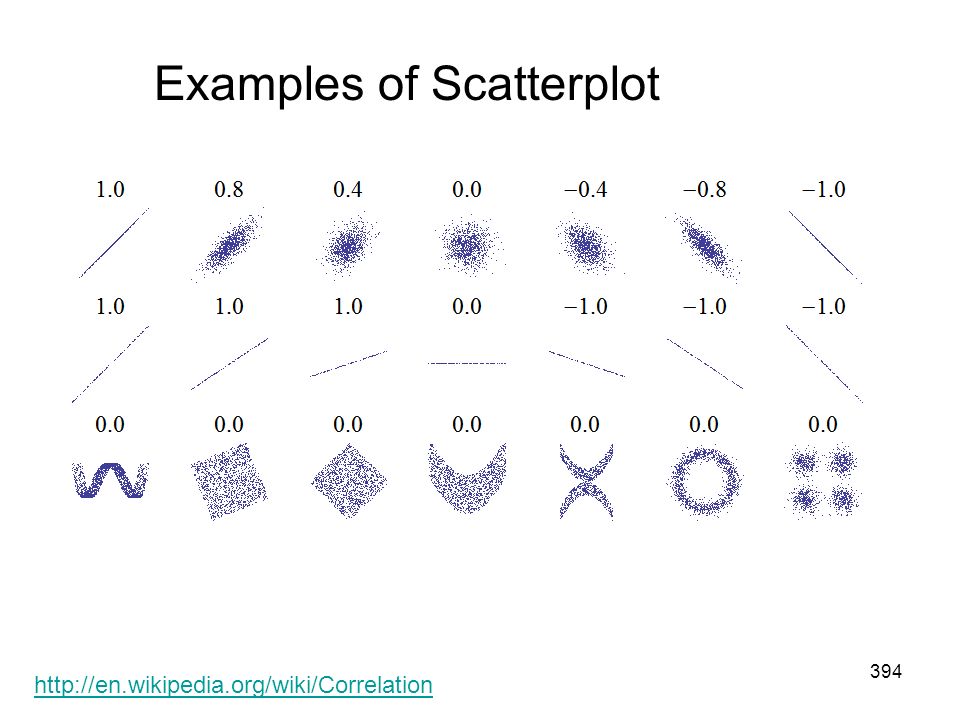
395
Linear Correlation Coefficient
The linear correlation coefficient, r, measures the strength of the linear association between the paired (x, y) values in a sample. The linear correlation coefficient is also referred to as the Pearson product moment or Pearson correlation coefficient in honor of Karl Pearson (1857 – 1936).
 values in a sample. The linear correlation coefficient is also referred to as the Pearson product moment or Pearson correlation coefficient in honor of Karl Pearson (1857 – 1936).")
396
Calculating the Linear Correlation Coefficient, r
Given paired data (x, y), as follows: x y x1 y1 x2 y2 . xn yn A positive r value indicates a positive association: as x increases (decreases), y increases (decreases). A negative r value indicates a negative association: as x increases (decreases), y decreases (increases). An r value close to +1 or -1 indicates a strong linear association. An r value close to 0 indicates a weak linear association.
, as follows: x. y. x1. y1. x2. y2. . xn. yn. A positive r value indicates a positive association: as x increases (decreases), y increases (decreases). A negative r value indicates a negative association: as x increases (decreases), y decreases (increases). An r value close to +1 or -1 indicates a strong linear association. An r value close to 0 indicates a weak linear association.")
397
Properties of Correlation
Always falls between -1 and +1 Sign of correlation denotes direction (-) indicates negative linear association (+) indicates positive linear association Correlation has a unitless measure - does not depend on the variables’ units Two variables have the same correlation no matter which is treated as the response variable Correlation is sensitive to outliers Correlation only measures strength of linear association.
 indicates negative linear association. (+) indicates positive linear association. Correlation has a unitless measure - does not depend on the variables’ units. Two variables have the same correlation no matter which is treated as the response variable. Correlation is sensitive to outliers. Correlation only measures strength of linear association.")
398
Calculating the Correlation Coefficient
Per Capita Gross Domestic Product and Average Life Expectancy for Countries in Western Europe Country Per Capita GDP (x) Life Expectancy (y) Austria 21.4 77.48 Belgium 23.2 77.53 Finland 20.0 77.32 France 22.7 78.63 Germany 20.8 77.17 Ireland 18.6 76.39 Italy 21.5 78.51 Netherlands 22.0 78.15 Switzerland 23.8 78.99 United Kingdom 21.2 77.37
 Life Expectancy (y) Austria Belgium Finland France Germany Ireland Italy Netherlands Switzerland United Kingdom")
399
Calculating the Correlation Coefficient
x y 21.4 77.48 -0.078 -0.345 0.027 23.2 77.53 1.097 -0.282 -0.309 20.0 77.32 -0.992 -0.546 0.542 22.7 78.63 0.770 1.102 0.849 20.8 77.17 -0.470 -0.735 0.345 18.6 76.39 -1.906 -1.716 3.271 21.5 78.51 -0.013 0.951 -0.012 22.0 78.15 0.313 0.498 0.156 23.8 78.99 1.489 1.555 2.315 21.2 77.37 -0.209 -0.483 0.101 = 21.52 = sum = 7.285 sx =1.532 sy =0.795 Z-Scores

400
Divide a Scatterplot into Quadrants
II In quadrant I, both z-scores positive; In quadrant II, z-scores of Internet are positive, while z-scores of GDP are negative; In quadrant III, both z-scores negative; In quadrant IV, z-scores of GDP are positive, while z-scores of INTERNET are negative; I IV III

401
R-Square, r2 When there is a correlation between x and y, we can express y in terms of x using a linear equation. The linear correlation coefficient, r, is often not 1 or – 1, indicating that the correlation is not perfect. The contribution of x to the variation in y can be measured by r2. The value of r2 is the proportion of the variation in y that is explained by the correlation between x and y. Example: The weights and heights of 10 bears are measured. The linear correlation coefficient r is Find what proportion of the variation in weights of bears can be explained by the correlation between the weights and heights of bears.

402
Using TI-83+ Calculators

403
Using Excel to Add a Trendline on Scatterplot
Step 1: Make the scatterplot Step 2: Right-click a data point, select “Add Trendline” and click on “Options” Check “Display Equation on Chart”. Check “Display R-squared value on Chart”. Step 3: Click on “Ok”.

404
Hypothesis Test for Correlation
H0: = 0 (there is no significant correlation) versus H1: ≠ 0 (there is a significant correlation) or H1: < 0 (there is a significant negative correlation) or H1: > 0 (there is a significant positive correlation) Test Statistic Make a decision using the classical method or P-value method.
 versus. H1: ≠ 0 (there is a significant correlation) or H1: < 0 (there is a significant negative correlation) or H1: > 0 (there is a significant positive correlation) Test Statistic. Make a decision using the classical method or P-value method.")
405
Example: The weights and heights of 10 bears are measured
Example: The weights and heights of 10 bears are measured. The linear correlation coefficient r is (a) Test the claim that there is a correlation between the weights and heights. Use = 0.05. (b) Test the claim that there is a positive correlation between the weights and heights. Use = 0.05.
 Test the claim that there is a correlation between the weights and heights. Use = (b) Test the claim that there is a positive correlation between the weights and heights. Use =")
406
Linear Regression: Introduction
Linear regression is one of the most important topics in statistics. Linear regression attempts to model the relationship between two variables by fitting a linear equation to observed data. One variable is considered to be an explanatory variable, and the other is considered to be a response variable (both quantitative).
.")
407
Introduction (cont’d)
(Linearity Check) Before attempting to fit a linear equation to observed data, a modeler should first determine whether or not there is a linear relationship between the variables of interest. A scatter-plot is a helpful tool in determining the strength of the relationship between two variables.
 Before attempting to fit a linear equation to observed data, a modeler should first determine whether or not there is a linear relationship between the variables of interest. A scatter-plot is a helpful tool in determining the strength of the relationship between two variables.")
408
The Linear Model Say we have a set of data, shown at the right. If we have reason to believe that there exists a linear relationship between the variables x and y, we can plot the data and draw a "best-fit" straight line through the data. That is, we can model the linear relationship by the familiar equation y = b0 + b1x. We can then find the slope, b1, and y-intercept, b0, for the data, which are shown in the figure below. x-axis: explanatory variable y-axis: response variable

409
Regression equation Least squares line

410
Some Concepts with Linear Regression
Predicted value: The estimate made from a model. Also known as fitted value and denoted Residual: the difference between the observed and the predicted values. Line of best fit: the line for which the sum of the squared residuals is the smallest.

411
A Picture Showing the Concepts
=

412
Least-Squares Method The most common method for fitting a regression line is the method of least-squares. This method calculates the best-fitting line for the observed data by minimizing the sum of the squared residuals (the vertical deviations from each data point to the line).
.")
413
Estimating the Regression Equation
If the scatterplot of data suggests a correlation, a straight line can be fitted to the data. The equation of such a line is determined by the least squares method and is found to be where

414
Estimating the Regression Equation: An Example
y 2 3 5 4 7 6 8 10 12

415
Residuals Revisited An observed data value can be represented as
Data = Model + Residual The standard deviation of the residuals is defined to be Not explained by the model

417
Interpreting Statistics: An Example
Researchers recorded facts about 77 breakfast cereals, including the calories and sugar content (in grams) of a serving. Suppose that, based on some data, the relationship between calories and sugar content can be modeled by and the R-square is Interpretation: The slope 2.50 says that cereals gain about 2.50 calories per gram of sugar. The intercept 89.5 predicts that sugar-free cereals would average about 89.5 calories. The R-square says that 31.8% of the variability in calories is accounted for by variation in sugar content.
 of a serving. Suppose that, based on some data, the relationship between calories and sugar content can be modeled by. and the R-square is Interpretation: The slope 2.50 says that cereals gain about 2.50 calories per gram of sugar. The intercept 89.5 predicts that sugar-free cereals would average about 89.5 calories. The R-square says that 31.8% of the variability in calories is accounted for by variation in sugar content.")
418
Predictions In predicting a value of y based on some given value of x ... If there is not a linear correlation, the best predicted y-value is the mean of y values. If there is a linear correlation, the best predicted y-value is found by substituting the x-value into the regression equation.

419
Using the Regression Equation for Prediction: Example1
Questions: If a country Per Captia GDP is $23,000, what is the life expectancy in that country? Life Expectancy = 0.42(23) = years
 = years.")
420
Using the Regression Equation for Prediction: Example2
Question: What does a regression line tell us the trend over the twentieth century? What does it predict about the mean annual temperature in year (i) 2005, (ii) 3000? When using the regression equation for predictions, stay within the scope of the available sample data.
 2005, (ii) 3000 When using the regression equation for predictions, stay within the scope of the available sample data.")
421
Is My Model Appropriate: Checking the Residual Plot
To see whether a model is appropriate, one plots the residuals against the predicted values. The model is appropriate, if the residuals show a horizontal direction, a shapeless form, and roughly equal scatter around 0-line for all predicted values. In short, a model is appropriate if the residual plot shows no pattern.

422
Model is appropriate

423
Model is bad

424
Variation and Prediction Intervals

425
Relationships (y - y) = (y - y) + (y - y)
(total deviation) = (explained deviation) + (unexplained deviation) (y - y) = (y - y) (y - y) ^ (total variation) = (explained variation) + (unexplained variation) (y - y) 2 = (y - y) (y - y) 2 ^
 = (explained deviation) + (unexplained deviation) (y - y) = (y - y) + (y - y) ^ (total variation) = (explained variation) + (unexplained variation) (y - y) 2 = (y - y) 2 + (y - y) 2. ^")
426
Coefficient of determination
explained variation. total variation The value of r2 is the proportion of the variation in y that is explained by the linear relationship between x and y.

427
Model Assumption The assumption underlying the regression model y = b0 + b1x + e: All error terms are independently and identically distributed as N(0, σ2).
.")
428
Estimate of the Error Variance σ2
y2 – b0 y – b1 xy n – 2

430
Prediction Interval (PI) for an Individual y
y - E < y < y + E ^ where E = t1-/2 se n(x2) – (x)2 n(x0 – x)2 1 n x0 represents the given value of x t1-/2 has n – 2 degrees of freedom
 – (x)2. n(x0 – x) n. x0 represents the given value of x. t1-/2 has n – 2 degrees of freedom.")
431
Prediction Interval (PI) for an Individual y: Example
Life Expectancy Find 95% PI for life expectancy for a country which has GDP per Capita is $25,000 se = 0.495 – < y < 77.06 < y <79.57

432
Inferences about Regression Coefficients
Confidence intervals Hypothesis tests

433
Multiple Regression

434
Chapter 10 Multinomial Experiments and Contingency Table
10-1 Overview 10-2 Multinomial Experiments: Goodness-of-Fit

435
Overview We focus on analysis of categorical (qualitative or attribute) data that can be separated into different categories (often called cells). A goodness-of-fit test is used to test the hypothesis that an observed frequency distribution fits (or conforms to) some claimed distribution. The hypothesis test will use the chi-square distribution with the observed frequency counts and the frequency counts that we would expect with the claimed distribution.
 some claimed distribution. The hypothesis test will use the chi-square distribution with the observed frequency counts and the frequency counts that we would expect with the claimed distribution.")
436
Definition Multinomial Experiment
This is an experiment that meets the following conditions: The number of trials is fixed. The trials are independent. All outcomes of each trial must be classified into exactly one of several different categories. The probabilities for the different categories remain constant for each trial. Multinomial experiments are extensions to the binomial experiment.

437
Multinomial Experiment: Example
Toss a die 300 times and record the outcome on each toss. This is a multinomial experiment because: The number of trials is fixed. (300 times) The trials are independent. All outcomes of each trial must be classified into exactly one of several different categories. (1, 2, 3, 4, 5, and 6) The probabilities for the different categories remain constant for each trial.
 The trials are independent. All outcomes of each trial must be classified into exactly one of several different categories. (1, 2, 3, 4, 5, and 6) The probabilities for the different categories remain constant for each trial.")
438
O represents the observed frequency of an outcome.
Goodness-of-Fit Test Notation O represents the observed frequency of an outcome. E represents the expected frequency of an outcome. k represents the number of different categories or outcomes. n represents the total number of trials.

439
Expected Frequencies

440
The Binomial Experiment
A special case of the multinomial experiment with k = 2. Categories 1 and 2: success and failure p1 and p2: p and q O1 and O2: x and n-x We made inferences about p: H0: p= p0 against H1: p≠ p0 In the multinomial experiment, we make inferences about the distribution; that is, all the probabilities, p1, p2, p3 …pk. ( H0: p1 = p10 , p2 = p20 , …, pk = pk0 , H1: at least one pi ≠ pi0 )
")
441
Goodness-of-Fit Test in Multinomial Experiments
Requirements: The data consist of a single sample that are randomly selected. The sample data consist of frequency counts for each of the different categories. For each category, the expected frequency is at least 5.

442
Goodness-of-Fit Test in Multinomial Experiments
H0: p1 = p10 , p2 = p20 , …, pk = pk0 against H1: at least one pi ≠ pi0 (called Goodness-of-Fit Test) Test Statistic where k = number of categories. Large values of the test statistic suggests rejection of the null hypothesis, so goodness-of-fit tests are always right-tailed.
 Test Statistic. where k = number of categories. Large values of the test statistic suggests rejection of the null hypothesis, so goodness-of-fit tests are always right-tailed.")
443
Goodness-of-Fit Test in Multinomial Experiments
A close agreement between observed and expected values will lead to a small value of 2 and a large P-value. A large disagreement between observed and expected values will lead to a large value of 2 and a small P-value. A significantly small P-value will cause a rejection of the null hypothesis of no difference between the observed and the expected.

444
Goodness-of-Fit Test in Multinomial Experiments: Example1
Toss a die 300 times with the following results. Is the die fair or biased? A multinomial experiment with k = 6 and O1 to O6 given in the table. We test: H0: p1= p2 = … = p6 = 1/6 (die is fair) H1: at least one pi is different from 1/6 (die is biased) Upper Face 1 2 3 4 5 6 Number of times 50 39 45 62 61 43
 H1: at least one pi is different from 1/6 (die is biased) Upper Face Number of times")
445
Goodness-of-Fit Test in Multinomial Experiments: Example1
Calculate the expected cell counts: Ei = npi = 300(1/6) = 50 Upper Face 1 2 3 4 5 6 Oi 50 39 45 62 61 43 Ei Test statistic and rejection region: Conclusion: There is insufficient evidence to indicate that the die is biased. What is the P-value?
 = 50. Upper Face Oi Ei. Test statistic and rejection region: Conclusion: There is insufficient evidence to indicate that the die is biased. What is the P-value")
446
Example: Fisher’s Reexamination of Mendel’s Data
Mendel crossed 556 smooth, yellow male peas with wrinkled, green female peas. According to now established genetic theory, the relative frequencies of the progeny should be as given in the following table. Observed Type Counts Smooth yellow Smooth green Wrinkled yellow Wrinkled green Relative Type Frequency Smooth yellow /16 Smooth green /16 Wrinkled yellow /16 Wrinkled green /16 Test that the observed counts come from a multinomial distribution with the prescribed probabilities.

447
Chapter 10 Multinomial Experiments and Contingency Table
10-3 Contingency Tables: Independence and Homogeneity

448
Key Concept In this section we consider contingency tables (or two-way frequency tables), which include frequency counts for categorical data arranged in a table with at least two rows and at least two columns. We present a method for testing the claim that the row and column variables are independent of each other. We will use the same method for a test of homogeneity, whereby we test the claim that different populations have the same proportion of some characteristics.
, which include frequency counts for categorical data arranged in a table with at least two rows and at least two columns. We present a method for testing the claim that the row and column variables are independent of each other. We will use the same method for a test of homogeneity, whereby we test the claim that different populations have the same proportion of some characteristics.")
449
Contingency Tables: Independence and Homogeneity
The experimenter measures two qualitative variables to generate bivariate data. For example, Gender and colorblindness Age and opinion Summarize the data by counting the observed number of outcomes in each of the intersections of category levels in a contingency table.

450
Layout of a r x c Contingency Table
A contingency table, having r rows and c columns—rc total cells, looks like this: 1 2 … c Total O11 O12 O1c r1 O21 O22 O2c r2 r Or1 Or2 Orc rr c1 c2 cc n

451
Definition Test of Independence
A test of independence tests the null hypothesis that there is no association between the row variable and the column variable in a contingency table. (For the null hypothesis, we will use the statement that “the row and column variables are independent.”) page 607 of Elementary Statistics, 10th Edition
 page 607 of Elementary Statistics, 10th Edition.")
452
Test of Independence Test Statistic Critical Value
Where O for observed cell frequency and E for expected cell frequency. Critical Value Found with chi-square table using degrees of freedom = (r – 1)(c – 1) r is the number of rows and c is the number of columns Larger test statistic values indicates rejection of independence, so tests of independence are always right-tailed. page 607 of Elementary Statistics, 10th Edition Same chi-square formula as for multinomial tables.
(c – 1) r is the number of rows and c is the number of columns. Larger test statistic values indicates rejection of independence, so tests of independence are always right-tailed. page 607 of Elementary Statistics, 10th Edition. Same chi-square formula as for multinomial tables.")
453
grand total = Total number of all observed frequencies in the table
Expected Frequency (row total) (column total) (grand total) E = grand total = Total number of all observed frequencies in the table page 607 of Elementary Statistics, 10th Edition
 (column total) (grand total) E = grand total = Total number of all observed frequencies in the table. page 607 of Elementary Statistics, 10th Edition.")
454
Expected Frequency for Contingency Tables
1 2 … j c Total O11 (E11=r1*c1/n) O12 (E12=r1*c2/n) O1c (E1c=r1*cc/n) r1 O21 (E21=r2*c1/n) O22 (E22=r2*c1/n) O2c (E2c=r2*c1/n) r2 i Oij Eij ri r Or1 (Er1=rr*c1/n) Or2 (Er2=rr*c2/n) Orc (Erc=rr*cc/n) rr c1 c2 cj cc n
 O12. (E12=r1*c2/n) O1c. (E1c=r1*cc/n) r1. O21. (E21=r2*c1/n) O22. (E22=r2*c1/n) O2c. (E2c=r2*c1/n) r2. i. Oij. Eij. ri. r. Or1. (Er1=rr*c1/n) Or2. (Er2=rr*c2/n) Orc. (Erc=rr*cc/n) rr. c1. c2. cj. cc. n.")
455
Example: BMD and Depression
In the paper “Depression and Bone Mineral Density: Is There a Relationship in Elderly Asian Men?” (Osteoporosis International, Vol. 16, pp ), S. Wong et al. pulished results of their study on BMD and depression for 1999 Hong Kong men aged 65 to 92 years. Here are the cross-classified data. Depression Osteoporiti Depressed Not depressed Total Low BMD 3 35 38 Normal 69 533 602 High BMD 97 1262 1359 169 1830 1999 BMD At the 5% significance level, do the data provide sufficient evidence to conclude that BMD and depression are statistically dependent for elderly Asian men?
, S. Wong et al. pulished results of their study on BMD and depression for 1999 Hong Kong men aged 65 to 92 years. Here are the cross-classified data. Depression. Osteoporiti. Depressed. Not depressed. Total. Low BMD Normal High BMD BMD. At the 5% significance level, do the data provide sufficient evidence to conclude that BMD and depression are statistically dependent for elderly Asian men")
456
Example: Disease and Blood Groups
Overfield and Klauber (1980) published the following data on the incidence of tuberculosis in relation to blood groups in a sample of Eskimos. Is there any association of the disease and blood group within the ABO system or within the MN system? Severity O A AB B Moderate-Advanced 7 5 3 13 Minimal 27 32 8 18 Not present 55 50 24 Severity MM MN NN Moderate-Advanced 21 6 1 Minimal 54 27 5 Not present 74 51 11
 published the following data on the incidence of tuberculosis in relation to blood groups in a sample of Eskimos. Is there any association of the disease and blood group within the ABO system or within the MN system Severity. O. A. AB. B. Moderate-Advanced Minimal Not present Severity. MM. MN. NN. Moderate-Advanced Minimal Not present")
457
Example: Political Affiliation and Attitude toward Testing of AIDS
A random sample of 500 persons were questioned regarding political affiliation and attitude toward government sponsored mandatory testing of AIDS. The results were as follows: favor Undecided Opposed Total Dem 135 80 65 280 Rep 95 60 220 230 140 130 500 Is there any association between political affiliation and attitude toward government sponsored mandatory testing of AIDS. ? Test at α=5%.

458
Limitation of Independence Tests
Rejection of independence implies an association between two qualitative variables, but strength of the association is unknown. Possible measures of association are relative risk odds ratio

459
Definition Test of Homogeneity
In a test of homogeneity, we test the claim that different populations have the same proportions of some characteristics. page 611 of Elementary Statistics, 10th Edition

460
How to Distinguish Between a Test of Homogeneity and a Test for Independence:
Were predetermined sample sizes used for different populations (test of homogeneity), or was one big sample drawn so both row and column totals were determined randomly (test of independence)? The key to identifying it is a test of homogeneity is the predetermined sample sizes.
, or was one big sample drawn so both row and column totals were determined randomly (test of independence) The key to identifying it is a test of homogeneity is the predetermined sample sizes.")
461
Example: Gene and Diabetes
Adult-onset diabetes is known to be highly genetically determined. A study was done comparing frequencies of a particular allele in a sample of such diabetics and a sample of nondiabetics. The data are shown below. Diabetic Normal Bb or bb BB Are the relative frequencies of the alleles significantly different in the two groups? Let p1 = p(BB|Diabetic) and p2 = p(BB|Normal). We need to test H0: p1 = p2, against H1: p1 ≠ p2.
 and. p2 = p(BB|Normal). We need to test H0: p1 = p2, against. H1: p1 ≠ p2.")
462
Can We Solve the Previous Problem Using the Two-Sample Proportion Test?
To test p1 = p2, the test statistic would be z, given by

463
Fisher Exact Test Fisher's exact test is a statistical test used to determine if there are nonrandom associations between two categorical variables. Often used when a 2X2 contingency table has a cell with an expected frequency less than 5. P-value is the probability of getting the observed results and more extreme. (Reject H0 if p-value ≤)
")
464
Fisher Exact Test a b c d 5 20 2 21 6 19 1 22 7 18 23 Table Table Table 3 Suppose we observed Table 1, and Table 2 and Table 3 are the more extreme cases. The p-value is the sum of the probability of observing those three tables.

465
Excel: Slide 15 Goodness-of-Fit Test in Multinomial Experiments
Find the expected values Click any empty cell Click button Select a Category: Statistical Select a function: CHITEST Type in Actual_range and Expected_range Click OK Returns the p-value.

466
Excel: Slide 15 Goodness-of-Fit Test in Multinomial Experiments

467
Excel: Slide 32 Test of Independence

468
SAS: Slide 15 Goodness-of-Fit Test in Multinomial Experiments
/*Goodness-of-Fit Test in Multinomial Experiments with equal probability Slide 15*/ DATA Die; input Dots $ count datalines; ; PROC freq data=die; weight count; tables dots / chisq; Run;

469
SAS Output: Slide 15 P-value

470
SAS: Pg515 Q2 Fisher Exact Test
Test of Independence ; Test of Homogeneity Fisher Exact Test /*Test of Independence; Test of Homogeneity Fisher Exact Test Text book page 515, question 2*/ DATA Helmet; input facial_injuries $ helmet $ number; datalines; yes yes 30 yes no 182 no yes 83 no no 236 ; PROC freq data=helmet; weight number; tables facial_injuries * helmet / chisq; run;

471
SAS Output: Pg515 Q2

472
Chapter 11 Analysis of Variance
11-1 Overview 11-2 One-Way ANOVA Copyright © 2007 Pearson Education, Inc Publishing as Pearson Addison-Wesley.

473
Hawkes Homework 11.1 and 11.2 12.1 Submit to D2L.

474
Preview Analysis of variance (ANOVA) is a technique for assessing how one or several nominal independent variables (called factors) affect a continuous dependent variable. ANOVA in which only one nominal independent variable is involved is called one-way ANOVA. ANOVA is usually employed in comparisons involving several population means. ANOVA is an extension to the independent-two-sample t test.
 is a technique for assessing how one or several nominal independent variables (called factors) affect a continuous dependent variable. ANOVA in which only one nominal independent variable is involved is called one-way ANOVA. ANOVA is usually employed in comparisons involving several population means. ANOVA is an extension to the independent-two-sample t test.")
475
Key Concept Analysis of variance is mainly used for tests of hypotheses that three or more population means are all equal against that at least one mean is different.

476
Overview Analysis of variance (ANOVA) is a method for testing the hypothesis that three or more population means are equal. For example: H0: µ1 = µ2 = µ3 = µk H1: At least one mean is different

477
ANOVA Methods Require the F-Distribution
1. The F- distribution is not symmetric; it is skewed to the right. 2. The values of F can be 0 or positive; they cannot be negative. 3. There is a different F-distribution for each pair of degrees of freedom for the numerator and denominator. Critical values of F are given in Table A-5

478
F - distribution

479
One-Way ANOVA Requirements
1. The populations have approximately normal distributions. 2. The populations have the same variance 2 (or standard deviation ). 3. The samples are simple random samples. 4. The samples are independent of each other.
. 3. The samples are simple random samples. 4. The samples are independent of each other.")
480
Procedure for testing Ho: µ1 = µ2 = µ3 = . . .
1. Construct an ANOVA table. 2. Identify the P-value. 3. Form a conclusion based on these criteria: If P-value , reject the null hypothesis of equal means. If P-value > , fail to reject the null hypothesis of equal means.

481
Procedure for testing Ho: µ1 = µ2 = µ3 = . . .
Caution when interpreting ANOVA results: When we conclude that there is sufficient evidence to reject the claim of equal population means, we cannot conclude from ANOVA that any particular mean is different from the others. There are several other tests that can be used to identify the specific means that are different, and those procedures are called multiple comparison procedures, and they are discussed later in this section.

482
Factors and Levels A nominal independent variable with k categories is called a factor with k levels. For example, to compare three different diets, A, B, and C, 60 people are available and are randomly assigned to the three diets so that each treatment group contains 20 people. Here diet is the only factor which has 3 levels. How to assign? Have slips of 20 A’s, 20 B’s, and 20 C’s in a bowl. Each person picks one.

483
H1: At least one of the means is different from the others.
Example: The following example studies the effect of bacteria on the nitrogen content of red clover plants. The (treatment) factor is bacteria strain, and it has six levels. Red clover plants are inoculated with the treatments, and nitrogen content is later measured in milligrams. 3DOK1 19.4 32.6 27.0 32.1 33.0 3DOK5 17.7 24.8 27.9 25.2 24.3 3DOK4 17.0 19.4 9.1 11.9 15.8 3DOK7 20.7 21.0 20.5 18.8 18.6 3DOK13 14.3 14.4 11.8 11.6 14.2 COMPOS 17.3 19.4 19.1 16.9 20.8 Question of interest: Do the effects of the 6 treatments differ significantly with regard to nitrogen content of red clover plants? We need to test H0: 1 = 2 = 3 = 4 = 5 = 6 H1: At least one of the means is different from the others.
 factor is bacteria strain, and it has six levels. Red clover plants are inoculated with the treatments, and nitrogen content is later measured in milligrams. 3DOK DOK DOK DOK DOK COMPOS Question of interest: Do the effects of the 6 treatments differ significantly with regard to nitrogen content of red clover plants We need to test. H0: 1 = 2 = 3 = 4 = 5 = 6. H1: At least one of the means is different from the others.")
484
Example: Five treatments for fever blisters, including a placebo, were randomly assigned to 30 patients. For each of the five treatments, the number of days from initial appearance of the blisters until healing is given as follows: Placebo 5 8 7 10 T1 4 6 3 5 T2 6 4 5 3 T3 7 4 6 3 5 T4 9 3 5 7 6 Questions of interest: Do the effects of the five treatments differ significantly with regard to healing fever blisters? Need to test H0: 1 = 2 = 3 = 4 = 5 vs. H1: At least one of the means is different from the others. Are the 4 treatments on average more effective than the placebo in healing fever blisters? Do the effects of the 4 treatments differ significantly with regard to healing fever blisters? If yes, which one is most effective?

485
Add the Analysis ToolPak to Excel 2007
Optional Add the Analysis ToolPak to Excel 2007 1. Click the Microsoft Office Button , and then click Excel Options. 2. Click Add-ins, and then in the Manage box, select Excel Add-ins. 3. Click Go. 4. In the Add-Ins available box, select the Analysis ToolPak check box, and then click OK.

486
Excel Optional Click Data Click Data Analysis Select Anova: Single Factor Click OK

487
Excel Select Input Range Check Labels in First Row Click OK

488
Excel Output P-value < , we reject the null hypothesis of equal means. There is sufficient evidence to support the claim that the four population means are not all the same.

489
Example: Growth of Soybeans
A plant physiologist investigated the effect of mechanical stress on the growth of soybean plants. Individually potted seedlings were randomly allocated to four treatment groups of 5 seedlings each. Seedlings in two groups were stressed by shaking for 20 minutes twice daily, while two control groups were not stressed. Also, plants were grown in either low or moderate light. Thus, the treatments were: Treatment 1: Low light, control Treatment 2: Low light, stress Treatment 3: Moderate light , control Treatment 4: Moderate light, stress After 16 days of growth, the plants were harvested and the total leaf area (cm2) of each plant was measured. The results are given in the next slide.
 of each plant was measured. The results are given in the next slide.")
490
Leaf Area of Soybean Plants
Treatment

491
Key Components of the ANOVA Method
SS(total), or total sum of squares, is a measure of the total variation (around x) in all the sample data combined. SS(total) = (x – x)2 page 644 of Elementary Statistics, 10th Edition
, or total sum of squares, is a measure of the total variation (around x) in all the sample data combined. SS(total) = (x – x)2. page 644 of Elementary Statistics, 10th Edition.")
492
Key Components of the ANOVA Method
SS(treatment), also referred to as SS(factor) or SS(between groups) or SS(between samples), is a measure of the variation between the sample means. SS(treatment) = n1(x1 – x)2 + n2(x2 – x) nk(xk – x)2 = ni(xi - x)2 page 644 of Elementary Statistics, 10th Edition
, also referred to as SS(factor) or SS(between groups) or SS(between samples), is a measure of the variation between the sample means. SS(treatment) = n1(x1 – x)2 + n2(x2 – x) nk(xk – x)2. = ni(xi - x)2. page 644 of Elementary Statistics, 10th Edition.")
493
Key Components of the ANOVA Method
SS(error), (also referred to as SS(within groups) or SS(within samples), is a sum of squares representing the variability that is assumed to be common to all the populations being considered. SS(error) = (n1 –1)s1 + (n2 –1)s2 + (n3 –1)s nk(xk –1)sk = (ni – 1)si page 644 of Elementary Statistics, 10th Edition 2
, (also referred to as SS(within groups) or SS(within samples), is a sum of squares representing the variability that is assumed to be common to all the populations being considered. SS(error) = (n1 –1)s1 + (n2 –1)s2 + (n3 –1)s nk(xk –1)sk. = (ni – 1)si. page 644 of Elementary Statistics, 10th Edition. 2.")
494
Key Components of the ANOVA Method
Given the previous expressions for SS(total), SS(treatment), and SS(error), the following relationship will always hold. SS(total) = SS(treatment) + SS(error) page 644 of Elementary Statistics, 10th Edition
, SS(treatment), and SS(error), the following relationship will always hold. SS(total) = SS(treatment) + SS(error) page 644 of Elementary Statistics, 10th Edition.")
495
MS(error) is a mean square for error, obtained as follows:
Mean Squares (MS) MS(treatment) is a mean square for treatment, obtained as follows: MS(treatment) = SS (treatment) k – 1 MS(error) is a mean square for error, obtained as follows: page 645 of Elementary Statistics, 10th Edition MS(error) = SS (error) N – k
 MS(treatment) is a mean square for treatment, obtained as follows: MS(treatment) = SS (treatment) k – 1. MS(error) is a mean square for error, obtained as follows: page 645 of Elementary Statistics, 10th Edition. MS(error) = SS (error) N – k.")
496
Test Statistic for ANOVA
MS (treatment) MS (error) Numerator df = k – 1 Denominator df = N – k page 645 of Elementary Statistics, 10th Edition
 MS (error) Numerator df = k – 1. Denominator df = N – k. page 645 of Elementary Statistics, 10th Edition.")
497
Class Exercise SS df MS F 4.500 16 27.425 19
Complete the ANOVA table SS df MS F Between Groups 4.500 Within Groups 16 Total 27.425 19 What are the null and alternative hypotheses? Identify the value of the test statistic. Find the critical value (Excel =finv(prob,df_numerator, df_denominator) Find the p-value (Excel =fdist(x,df_numerator, df_denominator) What can you conclude about the equality of the population means?
 Find the p-value (Excel =fdist(x,df_numerator, df_denominator) What can you conclude about the equality of the population means")
498
Identifying Means That Are Different
After conducting an analysis of variance test, we might conclude that there is sufficient evidence to reject a claim of equal population means, but we cannot conclude from ANOVA that any particular mean is different from the others. page 646 of Elementary Statistics, 10th Edition

499
Identifying Means That Are Different
Informal procedures to identify the specific means that are different Use the same scale for constructing boxplots of the data sets to see if one or more of the data sets are very different from the others. Construct confidence interval estimates of the means from the data sets, then compare those confidence intervals to see if one or more of them do not overlap with the others. page 646 of Elementary Statistics, 10th Edition

500
Bonferroni Multiple Comparison Test
Step 1. Do a separate t test for each pair of samples, but make the adjustments described in the following steps. Step 2. For an estimate of the variance σ2 that is common to all of the involved populations, use the value of MS(error). page 647 of Elementary Statistics, 10th Edition
. page 647 of Elementary Statistics, 10th Edition.")
501
Bonferroni Multiple Comparison Test
Step 2 (cont.) Using the value of MS(error), calculate the value of the test statistic, as shown below. (This example shows the comparison for Sample 1 and Sample 4.) page 647 of Elementary Statistics, 10th Edition
 Using the value of MS(error), calculate the value of the test statistic, as shown below. (This example shows the comparison for Sample 1 and Sample 4.) page 647 of Elementary Statistics, 10th Edition.")
502
Bonferroni Multiple Comparison Test
Step 2 (cont.) Change the subscripts and use another pair of samples until all of the different possible pairs of samples have been tested. Step 3. After calculating the value of the test statistic t for a particular pair of samples, find either the critical t value or the P-value, but make the following adjustment: page 647 of Elementary Statistics, 10th Edition
 Change the subscripts and use another pair of samples until all of the different possible pairs of samples have been tested. Step 3. After calculating the value of the test statistic t for a particular pair of samples, find either the critical t value or the P-value, but make the following adjustment: page 647 of Elementary Statistics, 10th Edition.")
503
Bonferroni Multiple Comparison Test
Step 3 (cont.) P-value: Use the test statistic t with df = N-k, where N is the total number of sample values and k is the number of samples. Find the P-value the usual way, but adjust the P-value by multiplying it by the number of different possible pairings of two samples. (For example, with four samples, there are six different possible pairings, so adjust the P-value by multiplying it by 6.) page 647 of Elementary Statistics, 10th Edition
 P-value: Use the test statistic t with df = N-k, where N is the total number of sample values and k is the number of samples. Find the P-value the usual way, but adjust the P-value by multiplying it by the number of different possible pairings of two samples. (For example, with four samples, there are six different possible pairings, so adjust the P-value by multiplying it by 6.) page 647 of Elementary Statistics, 10th Edition.")
504
Bonferroni Multiple Comparison Test
Step 3 (cont.) Critical value: When finding the critical value, adjust the significance level α by dividing it by the number of different possible pairings of two samples. (For example, with four samples, there are six different possible pairings, so adjust the α by dividing it by 6.) page 647 of Elementary Statistics, 10th Edition
 Critical value: When finding the critical value, adjust the significance level α by dividing it by the number of different possible pairings of two samples. (For example, with four samples, there are six different possible pairings, so adjust the α by dividing it by 6.) page 647 of Elementary Statistics, 10th Edition.")
505
Example

506
Calculating SS’s

507
Using the Bonferroni Test
Using the ANOVA table just obtained, we concluded that there is sufficient evidence to warrant rejection of the claim of equal means. The Bonferroni test requires a separate t test for each different possible pair of samples. page 648 of Elementary Statistics, 10th Edition

508
We begin with testing H0: μ1 = μ4 .
From the Table on slide 35: x1 = 25.9, n1 = 10, x4 = 19.6, n4 = 10 df = N – k = 40 – 4 = 36 Two-tailed P-value is , but adjust it by multiplying by 6 (the number of different possible pairs of samples) to get P-value = Because the adjusted P-value is less than α = 0.05, reject the null hypothesis. It appears that Samples 1 and 4 have significantly different means. Other tests can be conducted similarly. page 648 of Elementary Statistics, 10th Edition
 to get P-value = Because the adjusted P-value is less than α = 0.05, reject the null hypothesis. It appears that Samples 1 and 4 have significantly different means. Other tests can be conducted similarly. page 648 of Elementary Statistics, 10th Edition.")
509
11-3 Two-Way ANOVA

510
Key Concepts The analysis of variance procedure introduced in Section 11-2 is referred to as one-way analysis of variance because the data are categorized into groups according to a single factor (or treatment). In this section we introduce the method of two-way analysis of variance, which is used with data partitioned into categories according to two factors. page 655 of Elementary Statistics, 10th Edition
. In this section we introduce the method of two-way analysis of variance, which is used with data partitioned into categories according to two factors. page 655 of Elementary Statistics, 10th Edition.")
511
Two-Way Analysis of Variance
Two-Way ANOVA involves two factors. The data are partitioned into subcategories called cells. page 655 of Elementary Statistics, 10th Edition

512
Example: Diet and Weight Gain
A randomized experiment measured weight gain (in grams) of male rats under six diets varying by source of protein (beef, cereal, pork) and level of protein (high, low). Ten rats were assigned to each diet. The data are shown in the table below. Protein High Low Beef Cereal Pork page 655 of Elementary Statistics, 10th Edition Source
 of male rats under six diets varying by source of protein (beef, cereal, pork) and level of protein (high, low). Ten rats were assigned to each diet. The data are shown in the table below Protein. High Low. Beef. Cereal. Pork. page 655 of Elementary Statistics, 10th Edition. Source.")
513
Definition There is an interaction between two factors if the effect of one of the factors changes for different categories of the other factor. page 655 of Elementary Statistics, 10th Edition It is important to consider the interaction rather than just conducting another one-way ANOVA test on another factor.

514
Example: Diet and Weight Gain
Exploring Data: Calculate the mean for each cell. A randomized experiment measured weight gain (in grams) of male rats under six diets varying by source of protein (beef, cereal, pork) and level of protein (high, low). Ten rats were assigned to each diet. The data are shown in the table below. Protein High Low Beef Cereal Pork page 656 of Elementary Statistics, 10th Edition Source
 of male rats under six diets varying by source of protein (beef, cereal, pork) and level of protein (high, low). Ten rats were assigned to each diet. The data are shown in the table below Protein. High Low. Beef. Cereal. Pork. page 656 of Elementary Statistics, 10th Edition. Source.")
515
Example: Diet and Weight Gain
Exploring Data Display the means on a graph. If a graph results in line segments that are approximately parallel, we have evidence that there is not an interaction between the row and column variables. page 656 of Elementary Statistics, 10th Edition

516
Two-way ANOVA: requirements
1. For each cell, the sample values come from a population with a distribution that is approximately normal. 2. The populations have the same variance 2. 3. The samples are simple random samples. 4. The samples are independent of each other. 5. All of the cells have the same sample size. page 657 of Elementary Statistics, 10th Edition

517
Excel and TI-83/4 can be used.
Two-Way ANOVA calculations are quite involved, so we will assume that a software package is being used. Excel and TI-83/4 can be used.

518
Excel: Two-way ANOVA with Replication
Click Data Click Data Analysis Select: ANOVA: Two Factors With Replication Click OK Note: the data need to be in "unstacked" format.

519
Anova: Two-Factor With Replication

520
Using the 2-Way ANOVA Table
Step 1: Test for interaction between the effects: H0: There are no interaction effects. H1: There are interaction effects. The P-value is shown as > α = 0.05, so we fail to reject the null hypothesis of no interaction between the two factors.

521
Step 2: Check for Row/Column Effects (this step is necessary only if there is no interaction) :
H0: There are no effects from the row factors. H1: There are row effects. page 658 of Elementary Statistics, 10th Edition The P-value is shown as > α = 0.05, so we fail to reject the null hypothesis of no effects from source.

522
Step 2: Check for Row/Column Effects (this step is necessary only if there is no interaction):
H0: There are no effects from the column factors. H1: There are column effects. page 658 of Elementary Statistics, 10th Edition The P-value is shown as < α = 0.05, so we reject the null hypothesis of no effects from protein.

523
Special Case: One Observation per Cell and No Interaction
If our sample data consist of only one observation per cell, we lose MS(interaction), SS(interaction), and df(interaction). If it seems reasonable to assume that there is no interaction between the two factors, make that assumption and then proceed as before to test the following two hypotheses separately: page 659 of Elementary Statistics, 10th Edition H0: There are no effects from the row factors. H0: There are no effects from the column factors.
, SS(interaction), and df(interaction). If it seems reasonable to assume that there is no interaction between the two factors, make that assumption and then proceed as before to test the following two hypotheses separately: page 659 of Elementary Statistics, 10th Edition. H0: There are no effects from the row factors. H0: There are no effects from the column factors.")
524
Excel: Two-way ANOVA Without Replication
Click Data Click Data Analysis Select: ANOVA: Two Factors Without Replication Click OK Select Input Range Click OK

525
Excel Output: Two-way ANOVA Without Replication
Row factor: p-value =0.634, Fail to reject the null hypothesis. Column factor: p-value =0.598, Fail to reject the null hypothesis.

526
Class Exercise Complete the ANOVA table
Source SS df MS F P-value Factor A 415.87 Factor B 3 999.16 Interaction 117.88 Error 46 Total 57 Use a 0.05 significance level to test for an interaction between factor A and B Use a 0.05 significance level to test whether factor A is significant Use a 0.05 significance level to test whether factor B is significant

Similar presentations


