1. Introduction to Optimization Methods
MATLAB Optimization Toolbox

2. Presentation Outline Introduction Function Optimization
Optimization Toolbox
Routines / Algorithms available
Minimization Problems
Unconstrained
Constrained
Example
The Algorithm Description
Multiobjective Optimization
Optimal PID Control Example

3. Function Optimization
Optimization concerns the minimization or maximization of
functions
Standard Optimization Problem:
Subject to:
Equality Constraints
Inequality Constraints
Side Constraints
Where:
is the objective function, which measure and evaluate the performance of a system. In a standard problem, we are minimizing the function. For maximization, it is equivalent to minimization of the –ve of the objective function.
is a column vector of design variables, which can
affect the performance of the system.

4. Function Optimization (Cont.)
Constraints – Limitation to the design space. Can be linear or
nonlinear, explicit or implicit functions
Equality Constraints
Inequality Constraints
Most algorithm require less than!!!
Side Constraints

5. Optimization Toolbox
Is a collection of functions that extend the capability of MATLAB.
The toolbox includes routines for:
Unconstrained optimization
Constrained nonlinear optimization, including goal attainment
problems, minimax problems, and semi-infinite minimization
problems
Quadratic and linear programming
Nonlinear least squares and curve fitting
Nonlinear systems of equations solving
Constrained linear least squares
Specialized algorithms for large scale problems

6. Minimization Algorithm

7. Minimization Algorithm (Cont.)

8. Equation Solving Algorithms

9. Least-Squares Algorithms

10. Implementing Opt. Toolbox
Most of these optimization routines require the definition of an M-
file containing the function, f, to be minimized.
Maximization is achieved by supplying the routines with –f.
Optimization options passed to the routines change optimization
parameters.
Default optimization parameters can be changed through an
options structure.

11. Unconstrained Minimization
Consider the problem of finding a set of values [x1 x2]T that
solves
Steps:
Create an M-file that returns the function value (Objective
Function). Call it objfun.m
Then, invoke the unconstrained minimization routine. Use fminunc

12. Step 1 – Obj. Function function f = objfun(x)
f=exp(x(1))*(4*x(1)^2+2*x(2)^2+4*x(1)*x(2)+2*x(2)+1);
Objective function

13. Step 2 – Invoke Routine x0 = [-1,1];
Starting with a guess
x0 = [-1,1];
options = optimset(‘LargeScale’,’off’);
[xmin,feval,exitflag,output]=
fminunc(‘objfun’,x0,options);
Optimization parameters settings
Output arguments
Input arguments

14. Results
xmin =
feval =
1.3028e-010
exitflag = 1
output =
iterations: 7
funcCount: 40
stepsize: 1
firstorderopt: e-004
algorithm: 'medium-scale: Quasi-Newton line search'
Minimum point of design variables
Objective function value
Exitflag tells if the algorithm is converged.
If exitflag > 0, then local minimum is found
Some other information

15. More on fminunc – Input [xmin,feval,exitflag,output,grad,hessian]=
fminunc(fun,x0,options,P1,P2,…)
fun : Return a function of objective function.
x0 : Starts with an initial guess. The guess must be a vector
of size of number of design variables.
Option : To set some of the optimization parameters. (More after few slides)
P1,P2,… : To pass additional parameters.

16. More on fminunc – Output
[xmin,feval,exitflag,output,grad,hessian]=
fminunc(fun,x0,options,P1,P2,…)
xmin : Vector of the minimum point (optimal point). The size is the number of design variables.
feval : The objective function value of at the optimal point.
exitflag : A value shows whether the optimization routine is terminated successfully. (converged if >0)
Output : This structure gives more details about the optimization
grad : The gradient value at the optimal point.
hessian : The hessian value of at the optimal point

17. Options Setting – optimset
optimset(‘param1’,value1, ‘param2’,value2,…)
The routines in Optimization Toolbox has a set of default
optimization parameters.
However, the toolbox allows you to alter some of those
parameters, for example: the tolerance, the step size, the gradient
or hessian values, the max. number of iterations etc.
There are also a list of features available, for example: displaying
the values at each iterations, compare the user supply gradient or
hessian, etc.
You can also choose the algorithm you wish to use.

18. Options Setting (Cont.)
optimset(‘param1’,value1, ‘param2’,value2,…)
Type help optimset in command window, a list of options
setting available will be displayed.
How to read? For example:
LargeScale - Use large-scale algorithm if possible [ {on} | off ]
The default is with { }
Value (value1)
Parameter (param1)

19. Options Setting (Cont.)
optimset(‘param1’,value1, ‘param2’,value2,…)
LargeScale - Use large-scale algorithm if possible [ {on} | off ]
Since the default is on, if we would like to turn off, we just type:
Options = optimset(‘LargeScale’, ‘off’)
and pass to the input of fminunc.

20. Useful Option Settings
Highly recommended to use!!!
Display - Level of display [ off | iter | notify | final ]
MaxIter - Maximum number of iterations allowed [ positive integer ]
TolCon - Termination tolerance on the constraint violation [
positive scalar ]
TolFun - Termination tolerance on the function value [ positive
scalar ]
TolX - Termination tolerance on X [ positive scalar ]

21. fminunc and fminsearch
fminunc uses algorithm with gradient and hessian information.
Two modes:
Large-Scale: interior-reflective Newton
Medium-Scale: quasi-Newton (BFGS)
Not preferred in solving highly discontinuous functions.
This function may only give local solutions..
fminsearch is generally less efficient than fminunc for
problems of order greater than two. However, when the problem
is highly discontinuous, fminsearch may be more robust.
This is a direct search method that does not use numerical or
analytic gradients as in fminunc.
This function may only give local solutions.

22. Constrained Minimization
Vector of Lagrange
Multiplier at optimal point
[xmin,feval,exitflag,output,lambda,grad,hessian] = fmincon(fun,x0,A,B,Aeq,Beq,LB,UB,NONLCON,options,P1,P2,…)

23. Example
function f = myfun(x)
f=-x(1)*x(2)*x(3);
Subject to:

24. Example (Cont.)
For
Create a function call nonlcon which returns 2 constraint vectors [C,Ceq]
function [C,Ceq]=nonlcon(x)
C=2*x(1)^2+x(2);
Ceq=[];
Remember to return a null
Matrix if the constraint does
not apply

25. fmincon(fun,x0,A,B,Aeq,Beq,LB,UB,NONLCON,options,P1,P2,…)
Example (Cont.)
Initial guess (3 design variables)
x0=[10;10;10];
A=[ ;1 2 2];
B=[0 72]';
LB = [0 0 0]';
UB = [ ]';
CAREFUL!!!
fmincon(fun,x0,A,B,Aeq,Beq,LB,UB,NONLCON,options,P1,P2,…)

26. Example (Cont.) Const. 1 Const. 2 Const. 3 Const. 4 Const. 5 Const. 6
Warning: Large-scale (trust region) method does not currently solve this type of problem, switching to medium-scale (line search).
>
Optimization terminated successfully:
Magnitude of directional derivative in search direction less than 2*options.TolFun and maximum constraint violation is less than options.TolCon
Active Constraints: 2 9
x =
feval =
e-035
Const. 1
Const. 2
Const. 3
Const. 4
Const. 5
Const. 6
Const. 7
Sequence: A,B,Aeq,Beq,LB,UB,C,Ceq
Const. 8
Const. 9

27. Multiobjective Optimization
Previous examples involved problems with a single
objective function.
Now let us look at solving problem with multiobjective
function by lsqnonlin.
Example is taken for data curve fitting
In curve fitting problem the the error is reduced at each time step producing multiobjective function.

28. lsqnonlin in Matlab – Curve fitting
clc; %recfit.m
clear;
global data;
data= [
]; % experimental data,`1st coloum x, 2nd coloum R
x=data(:,1);
Rexp=data(:,2);
plot(x,Rexp,'ro'); % plot the experimental data
hold on
b0=[ ]; % start values for the parameters
b=lsqnonlin('recfun',b0) % run the lsqnonlin with start value b0, returned parameter values stored in b
Rcal=1./(1+exp(1.0986/b(1)*(x-b(2)))); % calculate the fitted value with parameter b plot(x,Rcal,'b'); % plot the fitted value on the same graph
Find b1 and b2
>>recfit
>>b =
%recfun.m
function y=recfun(b)
global data;
x=data(:,1);
Rexp=data(:,2);
Rcal=1./(1+exp(1.0986/b(1)*(x-b(2))));
% the calculated value from the model
%y=sum((Rcal-Rexp).^2);
y=Rcal-Rexp;
% the sum of the square of the difference
%between calculated value and experimental value
Link to this Page
Short tutorial Model Fitting last edited on 26 October 2003 at 7:22 pm by westlake.che.gatech.edu

29. Numerical Optimization
Newton –Raphson Method
Root Solver – System of nonlinear equations
(MATLAB – Optimization – fsolve)
2. One dimensional Solver –
(MATLAB - OPTIMIZATION Method )
Steepest Gradient Ascent/Descent Methods
Is the magnitude of descent direction.
achieve the steepest descent
achieve steepest ascent

30. Steepest Gradient Solve the following for two step steepest ascent
The partial derivatives can be evaluated at the initial guesses, x = 1 and y = 1,
Therefore, the search direction is –0.75i.
This can be differentiated and set equal to zero and solved for h* = Therefore, the result for the first iteration is x = 1 – 0.75(0.3333) = 0.75 and y = 1 + 0(0.3333) = 1. For the second iteration, the partial derivatives can be evaluated as,
Therefore, the search direction is –0.5625j.
This can be differentiated and set equal to zero and solved for h* = 0.25.
Therefore, the result for the second iteration is x = (0.25) = 0.75 and y = 1 + (–0.5625)0.25 =

31. %chapra … Contd
clear
clc
Clf x2
ww1=0:0.01:1.2;
ww2=ww1;
[w1,w2]=meshgrid(ww1,ww2);
J=-1.5*w1.^2+2.25*w2.*w1-2*w2.^2+1.75*w2;
cs=contour(w1,w2,J,70);
%clabel(cs);
hold
grid
w1=1; w2=1; h=0;
for i=1:10
syms h
dfw1=-3*w1(i)+2.25*w2(i);
dfw2=2.25*w1(i)-4*w2(i)+1.75;
fw1=-1.5*(w1(i)+dfw1*h).^ *(w2(i)+dfw2*h).*(w1(i)+…
dfw1*h)-2*(w2(i)+dfw2*h).^2+1.75*(w2(i)+dfw2*h);
J=-1.5*w1(i)^2+2.25*w2(i)*w1(i)-2*w2(i)^2+1.75*w2(i)
g=solve(fw1);
h=sum(g)/2;
w1(i+1)=w1(i)+dfw1*h;
w2(i+1)=w2(i)+dfw2*h;
plot(w1,w2) xi
pause(0.05)
End
MATLAB OPTIMIZATION TOOLBOX
w1(i), w2(i) function J=chaprafun(x)
w1=x(1);
w2=x(2)
J=-(-1.5*w1^2+2.25*w2*w1-2*w2^2+1.75*w2);
%startchapra.m
clc
clear
x0=[1 1];
options=optimset('LargeScale','off','Display','iter','Maxiter',… 20,'MaxFunEvals',100,'TolX',1e-3,'TolFun',1e-3);

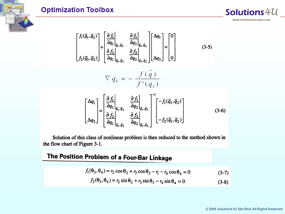
32. Newton –Raphson – Four Bar Mechanism
Sine and Cosine angle components - All angles referenced from global x - axis
In above equations θ1 = 0 as it is along the x-axis and other three angles are time varying.
1st angular velocity derivative

33. If input is applied to link2 - DC motor then ω2 would be the input to the syste
In Matrix for
2. Numerical Solution for Non Algebraic Equations

35. Newton-Raphson
%fouropt.m
function f=fouropt(x)
the = 0;
r1=12; r2=4; r3=10; r4=7;
f=-[r2*cos(the)+r3*cos(x(1))-r1*cos(0)-r4*cos(x(2));
r2*sin(the)+r3*sin(x(1))-r1*sin(0)-r4*sin(x(2))];
%startfouropt.m
clc
clear
x0=[ ];
options=optimset('LargeScale','off','Display','iter','Maxiter',… 200,'MaxFunEvals',100,'TolX',1e-8,'TolFun',1e-8);
theta3=x(1)*57.3
theta4=x(2)*57.3
Foursimmechm.m, foursimmech.mdl and possol4.m

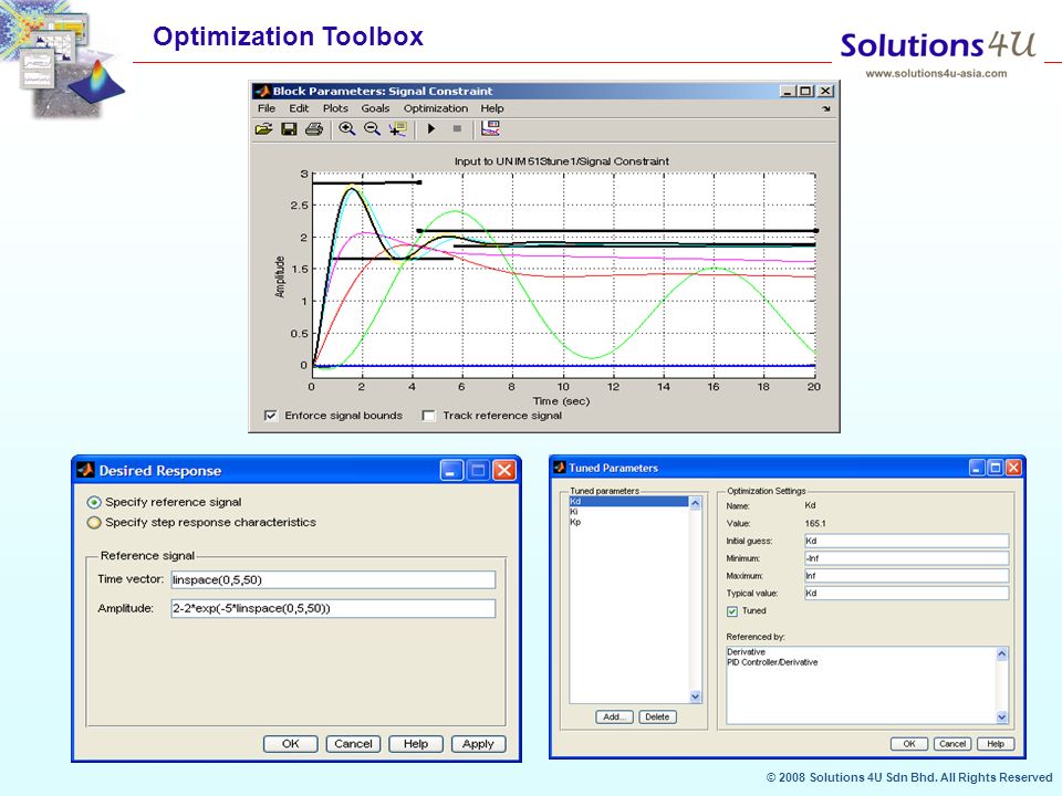
36. Simulink PID Controller Optimization
UNIM513tune1.mdl