1. Lecture 7 Transformations in frequency domain 1.Basic steps in frequency domain transformation 2.Fourier transformation theory in 1-D

2. 2 Basic steps for filtering in the frequency domain Takes spatial data and transforms it into frequency data The transformation is done by Fourier transformation The most common image transform takes spatial data and transforms it into frequency data

3. Complex numbers and expression a b R θ

4. Fourier series The Fourier transform is a method of expressing a periodic function with period 2T in terms of the sum of its projections onto a set of basis functions Fourier series: f(x) is periodic [-T, T]

5. Example of Fourier decomposition

6. Example by Maple =

7. Maple commands > f := piecewise(x < -1, x+2, x < 1, x, x < 3, x-2); > plot(f, x = -3..3, discont=true); > an := Int(x*cos(n*Pi*x), x = -1..1); > an := int(x*cos(n*Pi*x), x = -1..1); > bn := int(x*sin(n*Pi*x), x = -1..1); > with(plots): > F1 := plot(f, x = -3..3, discont=true, color=black): > S1 := sum(bn*sin(n*Pi*x), n = 1..1): > S2 := sum(bn*sin(n*Pi*x), n = 1..2): > S5 := sum(bn*sin(n*Pi*x), n = 1..5): > S20 := sum(bn*sin(n*Pi*x), n = 1..20): > F2 := plot({S1,S2,S5,S20}, x = -3..3): > display({F1,F2});

8. Fourier series in general form

9. Continue

10. Fourier transformation

11. Fourier series and Fourier transformation

12. Fourier Transform – 1D Fourier: Every periodic function f(x) can be decomposed into a set of sin() and cos() functions of different frequencies, given by F(u) is called the Fourier transformation of f(x). F(u) =R(u)+iI(u) repesents magnitudes cos and sin at frequency u. So we say F(u) is in the Frequency domain. Conversely, given F(u), we can get f(x) back using the inverse Fourier transformation

13. Fourier Spectrum Fourier decomposition: Fourier spectrum: Fourier phase: Decomposition:

14. Properties of Fourier transformation Linear

15. Fourier transformation and Convolution Convolution Theorem: assume then Proof

16. Example 1 Sinc(x)=sin(x)/x

17. Example 2 Impulse function and its Fourier transformation

18. Examples

19. Example: Discrete impulse function Unit discrete impulse function Impulse train function

20. Fourier transformation of impulse train

21. Sampling and FT of Sampled Function Sampled function

22. Sampling and FT of Sampled Function The value of each sample (strength of the weighted impulse)

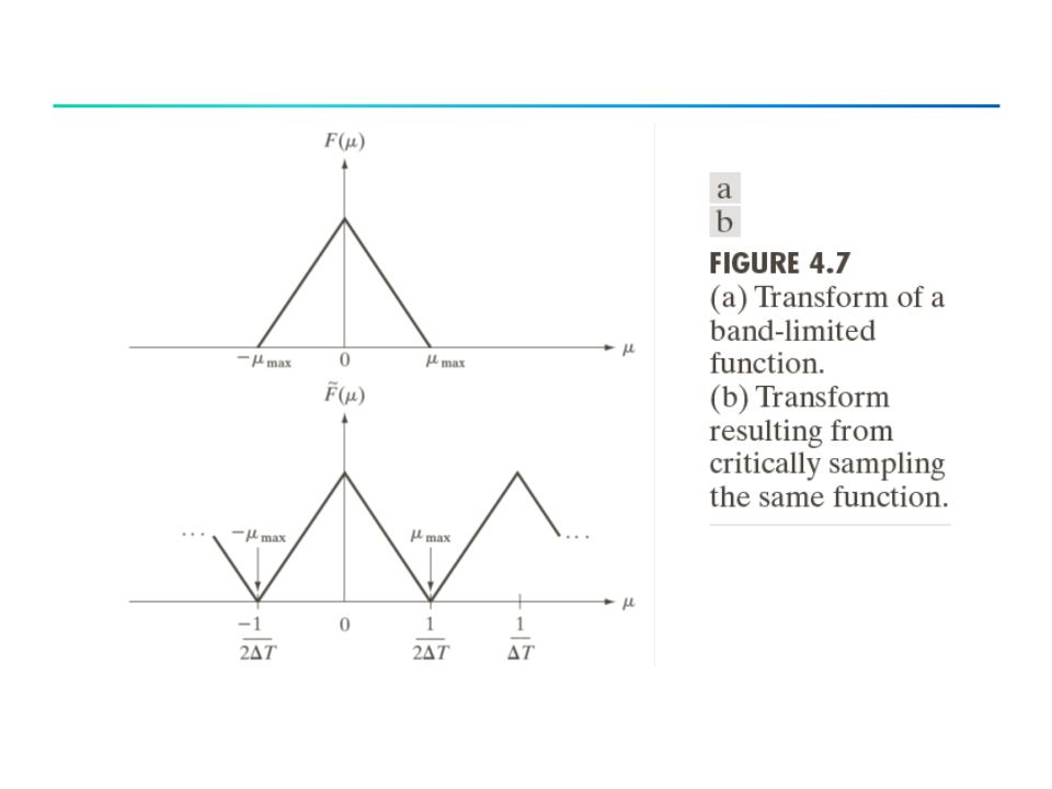
23. The Sampling Theorem Band-limited function f(t), its FT F(u) = 0 when u u max Let be the sampling function of f(t), and be its FT Question: if f(t) can be recovered from Sampling Theorem: if then f(t) can be recovered

24. The Sampling Theorem Sampling: –Over-sampling –Critically-sampling –Under-sampling Aliasing : f(t) is corrupted

27. Discrete Fourier Transform(DFT) Derive DFT from continuous FT of sampled function

28. DFT

29. Matrix representation

30. Example